Constant Coordinate Curves for Parabolic and Polar Coordinates
Constant Coordinate Curves for Parabolic and Polar Coordinates

This Demonstration shows curves of constant coordinate values for the parabolic and polar coordinate systems in two dimensions. As you drag the locator in the plane, the curves are redrawn so they pass through that point. Holding the mouse over the curve shows which variable is constant along that curve, and holding it over the point gives the actual values of the variables. For comparison, the Cartesian coordinate system is also included.
xy
Details
Details
Polar coordinates may be defined by , , for , . The inverse relation is , . Note that is indeterminate at the origin
(r,θ)
x=rcos(θ)
y=sin(θ)
r∈[0,∞)
θ∈(-π,π]
r=+
2
x
2
y
θ=(x,y)
-1
tan
θ
(x,y)=(0,0).
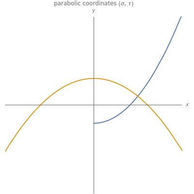
Parabolic coordinates may be defined by , , for , . The inverse relation is , , where is the unit step function.
(σ,τ)
x=στ
y=(-)/2
2
τ
2
σ
σ∈(-∞,∞)
τ∈[0,∞)
σ=(2θ(x)-1)+-y
2
x
2
y
τ=++y
2
x
2
y
θ(x)
Note that most descriptions of parabolic coordinates do not include the term and restrict the domain of to . However, this is ambiguous since the two points then map to the same . By including the term we avoid this ambiguity so that corresponds to the left half-plane and to the right half-plane.
θ(x)
σ
σ∈[0,∞)
(±x,y)
(σ,τ)
θ(x)
σ<0
σ≥0
External Links
External Links
Permanent Citation
Permanent Citation
Peter Falloon
"Constant Coordinate Curves for Parabolic and Polar Coordinates"
http://demonstrations.wolfram.com/ConstantCoordinateCurvesForParabolicAndPolarCoordinates/
Wolfram Demonstrations Project
Published: March 7, 2011