ABSTRACT (original article): The present study develops a flexible and interactive decision‑support application for portfolio optimization, grounded in Modern Portfolio Theory and implemented within the Mathematica computational environment. The tool enables users to construct, analyze, and evaluate investment portfolios dynamically, incorporating real-time sensitivity analysis. In accordance with contemporary portfolio theory, it integrates two principal optimization strategies: (a) the Minimum Variance Portfolio and (b) the Maximum Sharpe Ratio Portfolio. The computational framework ingests real stock market data (Yahoo Finance), from which returns and covariance matrices are calculated. The resulting data serves as inputs for solving the corresponding optimization problems under user‑defined constraints. A key feature of the tool is the ability to perform real‑time sensitivity analysis with respect to expected returns, as well as to interactively adjust the risk‑aversion coefficient, providing users with immediate visual and numerical feedback. Interpretability is enhanced through graphical representations of the Efficient Frontier, overlaid with the optimal portfolios and the Capital Market Line on a unified plot. These visualizations support both educational and practical financial decision‑making. Overall, the tool offers a novel contribution by offering a hands‑on, visually rich, and analytically rigorous environment for understanding and applying portfolio optimization methods using real‑world data. CITATION (original article): Pelekoudas, C. M., Tsopouridou, E. P., & Papadopoulos, I. (2025). An Application for Portfolio Optimization, Risk Sensitivity and Efficient Frontier Visualization in Mathematica. Digital Technologies Research and Applications, 4(2), 212–231. https://doi.org/10.54963/dtra.v4i2.1364
This notebook focuses on the Efficient Frontier, a central concept in modern portfolio theory (MPT). The Efficient Frontier represents the set of portfolios that achieve the best possible trade-off between expected return and risk: for a given level of risk, it delivers the highest return, while for a given level of return, it achieves the lowest possible risk.
Using computational tools from the Wolfram Language, the notebook demonstrates how expected returns, variances, and correlations between assets can be estimated, and how optimization techniques are applied to identify portfolios along the Efficient Frontier.
The aim is to present both the theoretical foundation of portfolio optimization and its practical application, highlighting how mathematical and computational methods can support investment decision-making.
1. User Login
1. User Login
In[]:=
cols=Input["How many assets do you want to import?"];(*Numberofsharestoanalyze*)startdate=Input["Enter start date (e.g. \"Jan.1,2025\"): "];(*Datastartdate*)enddate=Input["Enter end date (e.g. \"Feb.1,2025\"): "];(*Dataenddate*)lmax=Input["Maximum risk aversion λ (e.g. 3):"];(*Upperlimitofriskaversioncoefficient*)rf=Input["Risk-free rate rf (e.g. 0.02):"];(*Fixedrisk-freerate*)
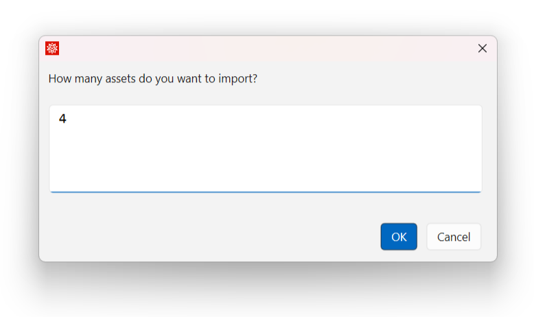
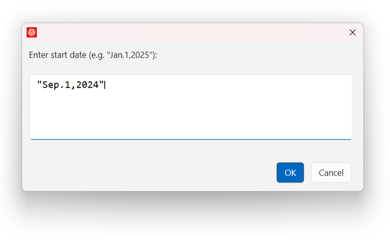
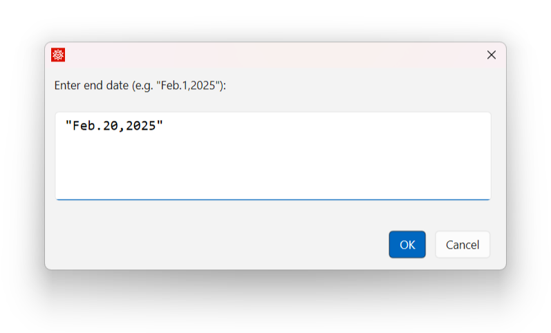
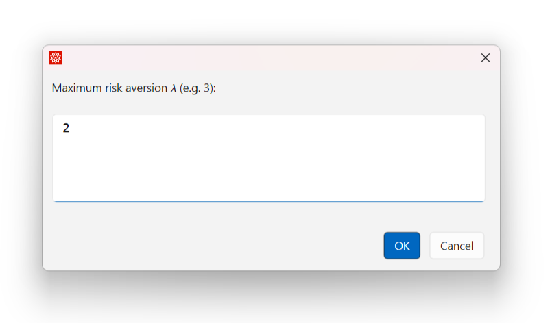
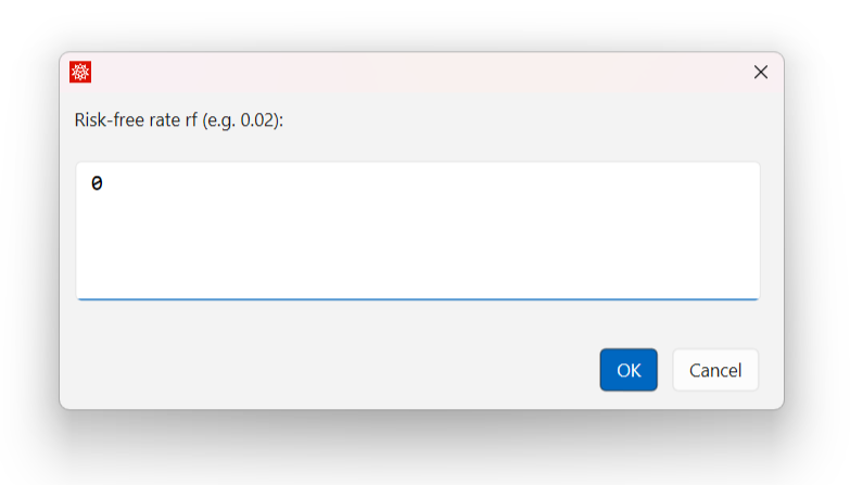
Importing titles of assets
In[]:=
tickers={};Do[AppendTo[tickers,Input["Enter ticker for asset "<>ToString[i]<>"(e.g. \"GOOG\"): "]],{i,1,cols}];
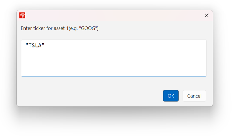
2. Financial Data Recovery
2. Financial Data Recovery
In[]:=
allData={};Do[Module[{m,t},m=FinancialData[ticker,{startdate,enddate}];(*Historicalpricedata*)t=Which[Head[m]===TemporalData,m["Values"],(*TemporalDataobject*)Head[m]===TimeSeries,m["Values"],(*TimeSeriesobject*)Head[m]===List&&Length[m]>0&&Head[m[[1]]]===List,Last/@m,(*Listof{date,price}pairs*)Head[m]===Missing,Print["Missing data for ",ticker];{},(*Missingdata*)Head[m]===$Failed,Print["Failed to get data for ",ticker];{},(*Failedrequest*)True,Print["Unexpected format for ",ticker,": ",Head[m]];{}(*Unknownformat*)];If[Length[t]>0,AppendTo[allData,t],Print["No data available for ",ticker]];],{ticker,tickers}];
3. Returns & Co-variation Calculations
3. Returns & Co-variation Calculations
In[]:=
matrix=Transpose[allData];(*Pricetableperday*)rows=Length[matrix];
Calculating percentage daily returns
In[]:=
matrix2=Table[(matrix[[i+1,j]]-matrix[[i,j]])/matrix[[i,j]],{i,1,rows-1},{j,1,cols}];
In[]:=
mo=Table[Mean[matrix2[[All,j]]],{j,1,cols}];(*Averagereturnofeachasset*)cov=Transpose[matrix2].matrix2/(rows-1);(*Covariancetable*)w=Table[Symbol["w"<>ToString[i]],{i,1,cols}];(*Weightvariablesforoptimization*)
4. Interactive Optimization & Presentation
4. Interactive Optimization & Presentation
In[]:=
ManipulateModule{e,s2,con,min1,risk1,weights1,sharpe1,returns1,cum1,min2,sharpeVal,weights2,sharpe2,returns2,cum2,avplus,avminus,minplus1,minminus1},(*Constraints:Sumofweights=1andnonegativeweights*)con=Join[{Total[w]1},Table[0≤w[[i]]≤1,{i,1,cols}]];e=mo.w;(*Expectedportfolioreturn*)s2=w.cov.w;(*Portfoliovariation*)(*MODEL1:MINIMUMVARIATION*)min1=Minimize[{s2-l*e,con},w];(*Minimizingobjectivefunction*)risk1=weights1.cov.weights1;(*Objectivefunctionvalue*)weights1=Chop[w/.min1[[2]],10^-10];(*Optimalweights*)sharpe1=(mo.weights1-rf)Sqrt[weights1.cov.weights1];(*Sharperatio*)returns1=matrix2.weights1;cum1=FoldList[Times,1,1+returns1];(*Cumulativeperformanceperday*)(*SENSITIVITYANALYSIS(ONLYforMinVariance)*)avplus=(1+sensit)*mo;(*IncreaseaveragereturnsbyX%*)avminus=(1-sensit)*mo;(*DecreaseaveragereturnsbyX%*)minplus1=Minimize[{w.cov.w-l*(avplus.w),con},w];minminus1=Minimize[{w.cov.w-l*(avminus.w),con},w];(*MODEL1:MAXIMUMSHARPERATIO*)min2=Minimize[{-(e-rf)/Sqrt[s2],con},w];(*Sharpetargetreversalforminimization*)sharpeVal=min2[[1]];weights2=Chop[w/.min2[[2]],10^-10];(*OptimalweightsformaximumSharpe*)sharpe2=(mo.weights2-rf)Sqrt[weights2.cov.weights2];returns2=matrix2.weights2;cum2=FoldList[Times,1,1+returns2];(*PresentationofResults*)Column[{Style["Model 1: Minimum Variance",Bold,Blue],Grid[{{"Risk (σ²):",risk1},{"Sharpe Ratio:",NumberForm[sharpe1,{3,3}]},{"Weights:",Grid[Transpose@{tickers,weights1},FrameAll]},{"+Sensit [%]:",sensit*100,"→",minplus1[[1]]},{"-Sensit [%]:",sensit*100,"→",minminus1[[1]]},{"Cumulative Return:",ListLinePlot[cum1,PlotStyleRed,AxesLabel{"Day","Return"},ImageSizeMedium]}}],Spacer[15],Style["Model 2: Maximum Sharpe",Bold,Darker@Green],Grid[{{"Sharpe Ratio (max):",NumberForm[sharpe2,{3,3}]},{"Risk (σ²):",weights2.cov.weights2},{"Weights:",Grid[Transpose@{tickers,weights2},FrameAll]}}]}],{{l,0,"Risk Aversion Coefficient λ"},0,lmax,0.01},{{sensit,0.05,"Sensitivity ± (%)"},0,0.1,0.01},SaveDefinitions->True
1. Creating a range of values for the risk aversion coefficient λ
2. Setting restrictions on asset weights
3. Calculate Efficient Frontier for each λ
4. Calculating Max Sharpe Portfolio
5. Minimum Variance Portfolio Calculation
6. Construct Capital Market Line as a list of points
7. Drawing a Graph with a Legend
8. Weighting Tables for the two main portfolios
9. Final Presentation (graph and weights together)
CITE THIS NOTEBOOK
CITE THIS NOTEBOOK
An application for portfolio optimization, risk sensitivity and efficient frontier visualization in Mathematica
by Charalampos M. Pelekoudas, Eleni P. Tsopouridou & Ioannis Papadopoulos
Wolfram Community, STAFF PICKS, September 25, 2025
https://community.wolfram.com/groups/-/m/t/3551033
by Charalampos M. Pelekoudas, Eleni P. Tsopouridou & Ioannis Papadopoulos
Wolfram Community, STAFF PICKS, September 25, 2025
https://community.wolfram.com/groups/-/m/t/3551033