Wolfram Cloud Document

This notebook series is designed to introduce selected dynamic economic models to both advanced undergraduate and graduate students. Economists have relied on a series of economic models to better understand the otherwise highly complex causal relationship among many economic variables. Dynamic economic models set up by systems of either difference or differential equations are particularly useful in tracing the change in the quantity of unknown economic variables (e.g., the capital stock, demand for labor, aggregate output, etc.) and their interactions over time.

This notebook series aims to help students better understand the depth, usefulness, and limitations of major existing micro and macroeconomic models by demonstrating how we can use Wolfram Mathematica to replicate and reconstruct the core ideas and find dynamic solution of the model.

The model introduced in this notebook series include, among others, (1) the cobweb model of the quantity and price adjustment, (2) Keynes’s aggregate demand model, (3) Hicks’s ISLM model, (4) Samuelson’s investment accelerator model, (5) Kalecki’s investment delay model, (6) the predator-prey interaction model, (7) the epidemic model, (8) Ricardo’s three dimensional business cycle model, (9) Marx-Goodwin business cycle and growth model, (10) Smith’s and Ricardo’s growth model, (11) the Harrod-Domar growth model, (12) the Solow growth model, (13) the RBC model, (14) Romer’s new growth model, and (15) the circuit of capital model.

Dynamic inflation models III

Keynesian cost of production approach to inflation

Introduction

Against this backdrop, Keynes presented his cost of production theory of inflation in Book V of General Theory. Keynes blames that classical economists have never properly articulated a coherent theory of price: At one point, they use the supply and demand analysis to explain the change in the price of a product; at other times, they also talk about the quantity of money in circulation determining the price level in the economy. In the latter case, however, classical economists have never properly explained how exactly the change in the quantity of money affects the overall price level.

Following Keynes’s reasoning, let us think about the following scenario: What would happen if central bank (assuming that it is the only institution that determines the quantity of money in circulation and the related terms of borrowing money in the economy) substantially increases the quantity of money? Would this monetary policy decision inevitably increase the overall price level in the economy? Yes, according to classical economists. But how and why? Would this belief be still valid even when major private economic agents (e.g., individuals, non-financial firms, and private banks) continue to hoard this increased quantity of money on their financial balance for meeting their precautionary purposes? What abut the case when some economic agents (e.g., individuals and financial companies) hold a significant portion of this increased quantity of money to meet their speculative motive for holding liquidity? Wouldn’t this create a financial bubble instead of increasing the price level?

Keynes argues that the classical quantity of money theory of inflation fails to answer these questions and their argument can be made sense only when we assume a special case in which the economy is fully utilizing its productive resource and and in which there is no precautionary and speculative motive for holding money. Unlike what classical monetarists assumed away, central bank’s expansionary monetary policy only translates itself into what Keynes calls ‘liquidity trap’ in the face of strengthened precautionary motive for holding money. The same monetary policy can create a financial asset bubble rather than increasing the price level and inflation.

As an alternative to this partial theory, Keynes argues that the macroeconomic price level and its change can and must be explained by the changing cost structure that enters the production process in the economy. Of course, there are many factors of production, and the price of these input factors can change over time as various monetary and non-monetary macroeconomic variables change. Nonetheless, if there is an upward pressure for the rising price of any input, there will be a corresponding increase in the price of the final goods and services and its rate of change.

In this section, we summarize Keynes’s cost of production theory of inflation and contrast his theory with modern-day monetarist revivals of the classical quantity of money theory of inflation. As a special case, we will also discuss how to model the price behavior when the economy is stimulated too much moving beyond its full employment range. The second part of analysis is to model the price and wage interaction assuming that the the economy is pushed to operate at this wage - price spiral domain.

The behavior of changing input prices over the business cycle and the classical money-price causality

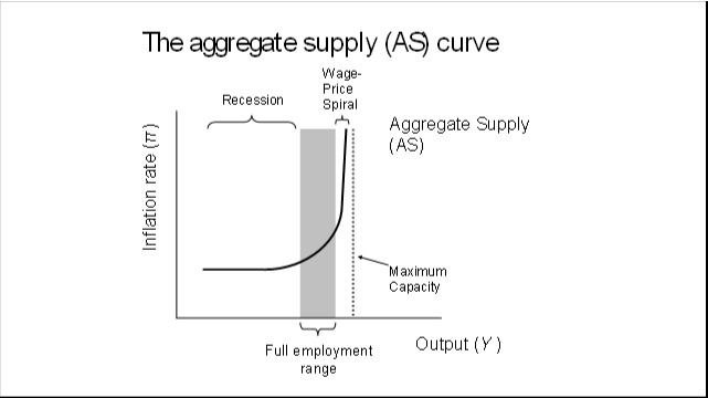
From Keynes' s point of view, the private economy can be operated at the following three distinct domains : (1) The first domain is what Keynes calls ' less than full employment range . ' (2) The second domain is the full employment range, in which various factors of production are fully utilized. If the economy is stimulated further moving beyond this full employment range, we can call this state (3) ' wage - price spiral range.' Keynes observes that the price of various input changes over time depending on which state the economy is operating at.

If the economy is in a severe recession (less than full employment range), the price of various input tends to fall. In the worse case, the economy will experience a prolonged deflationary danger. Under these circumstances, a carefully designed expansionary fiscal and monetary policy can substantially alleviate socioeconomic problems associated with prolonged unemployment and/or under-utilization of productive resources; it can also rapidly increase aggregate demand and output via investment-output multiplier channel. Under this particular state of the economy, neither expansionary fiscal policy nor monetary policy would be inflationary.

When the economy is operating near the full employment range, however, the price of various input tends to rise rapidly as the competitive demand for these input from various sectors drive up the cost of production in final goods producing sectors of the economy. Under these circumstances, if both fiscal and monetary authority continuously adopt unabated expansionary policies it will end up creating ‘true (monetary) inflation phenomenon.’ Rather than increasing aggregate output-income, an increase in the quantity of money increase the price level of the economy in exact proportion.

To fully analyze this nonlinear dynamical interaction between the change in aggregate output-income and the price level, Keynes draws our attention to the following behavior of input price over the business cycle:

◼

Factors of production and resources are not homogeneous. Both capital goods and labor are heterogeneous and retain a varying degree of productivity and/or skills. Therefore, the changing demand for the individual factors and resources and their price vary across the industry and firm, and their demand and prices may move in opposite direction even when the economy is in recession;

◼

The output-input ratio, the ratio of output-capital and of output-labor may fall as the economy moves toward the full employment level. Therefore, there is diminishing, and not constant, returns in the productivity of input as employment and utilization of them gradually increases. Because of varying ratios, the demand and price of various input can rise even before the economy reaches full employment range;

◼

Some factors of production and resources are not freely interchangeable. Thus, depending on the technical composition of production unit (the ratio between non-labor and labor input ), some inputs and intermediate goods may reach a condition of inelastic supply, while there are still unemployed resources available for producing other goods even before the economy reaches its full employment level;

◼

The nominal wage tends to rise, even before the economy reaches full employment level. Though Keynes did not explain this much, perhaps he was assuming a sufficiently powerful bargaining power retained by workers and labor unions in some crucial industrial sectors that might exercise their collective bargaining power to either retain or demand a higher nominal wage even in a recession period;

◼

The relative income accruing to various owners of factors of production may not all change in the same direction. Even when the economy is recovering from the recession or underemployment situation, wages for workers and prices of intermediate goods used in a particular industry and firm may fall, not rise, against the overall trend. For these reasons, both labor and non-labor cost can vary in opposite directions along the business cycle (Keynes 1997: 296).

Due to these complex factors and their changing price behaviors, “instead of [having] constant prices in conditions of unemployment, and of prices rising in proportion to the quantity of money in conditions of full employment, we have in fact a condition of prices rising gradually as employment increases” [well before the economy reaches its full employment capacity] (Keynes 1997: 297).

Economists have to carefully weigh varying effects of the changes in the quantity of money on both effective demand and price level. We “must first consider the effect of changes in the quantity of money on the size of effective demand; and the increase in effective demand will spend itself partly in increasing the quantity of employment and partly in raising the level of price.”(Ibid)

In sum, classical economists’ simple and unidirectional causality between the change in the quantity of money and the change in the price level irrespective of the state of the economy fails to explain the true cause of inflation phenomenon at a given period.

The effect of expansionary monetary policy on aggregate output and the price level over the business cycle

Of course, the change in the quantity of money and/or the related terms of borrowing (interest rate) can have an impact on both aggregate demand and the general price level. The increase in the quantity of money may have a positive effect on increasing effective demand via a high interest-rate sensitivity of investment, while at the same time on raising the price level.

Exactly which aspect and channel is pronounced will depend on how the change in the quantity of money affects the rate of interest and investment, and how the increase in employment is induced by the increase in private business investment spending. It also depends on the relationship between the capital goods sector and the consumer goods sector that are making business transactions for securing capital equipment. How individual workers in different industrial sectors will respond to the rising price level and falling real wage also influence this channel.

In general, however, we can say that if the economy is operating far below its full capacity, the increase in the quantity of money will have a greater impact on increasing aggregate demand and output than on inflation (assuming the public’s propensity to consume and liquidity preference remain the same as before, which is highly unlikely if the recession is prolonged). As the economy slowly reaches its full employment, on the other hand, the increase in the quantity of money would have less positive impact on increasing aggregate demand and output, but more impact on the level of price.

“When a further increase in the quantity of effective demand produces no further increase in output, and [the increase in the quantity of money] entirely spends itself on an increase in the cost-unit [weighted average of cost of production] fully proportionate to the increase in effective demand,” there will be a true inflation, the rise in the price level in exact proportion of the increase in the quantity of money.

“Up to this point, [however,] the effect[iveness] of monetary expansion [on increases in output and employment] is entirely a question of degree, and there is no previous point at which we can draw a definite line and declare that conditions of inflation have set in. Every previous increase in the quantity of money is likely, in so far as it increases effective demand,” to partly increase the cost unit and partly increase output.

From this perspective, the classical economic theory is simply assuming that the economy is always operating at its full employment level. From their point of view, any increase in the quantity of money directly and proportionately increases the price level, without having any positive effect on aggregate demand and output. “The view that any increase in the quantity of money is inflationary --- is bound up with the underlying assumption of the classical theory that we are always in a condition [of full employment and] where a reduction in the rewards of the factors of production will lead to a curtailment in their supply [Say’s law: the supply always creates its own demand].”(Keynes 1997: 304)

Modern-day advocates of the quantity of money theory of inflation (Monetarists, New Classical School, and Real Business Cycle School), therefore, (1) propose restrictive monetary policy rules that prohibit the government and central bank’s counter-cyclical expansionary monetary policies and (2) justify the institutional arrangement for this restrictive monetary policy rule in the name of ‘central bank independence’ and/or ‘inflation targeting.’ As soon as we attempt to apply any policy drawn from this classical view, it becomes completely irrelevant and even disastrous from Keynes’s perspective.

Keynes’s nonlinear inflation rate dynamics and system dynamic simulation

Keynes’s cost of production approach to the price level and inflation rate can be roughly captured by the following graphical illustration:

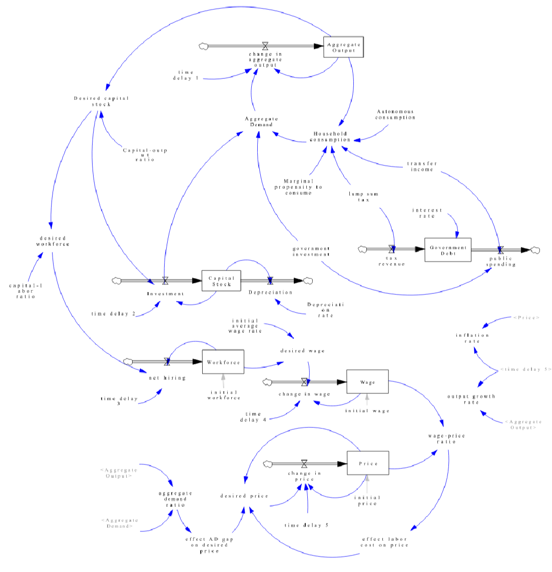
Using a System Dynamics modeling software, Vensim, we can create the following stock-flow diagram that shows the connection among the change in private business investment spending, the government’s expenditure, aggregate demand, aggregate output-income, on the one hand, and their relationship with the changing demand for labor, nominal wages and the price level in a hypothetical economy:

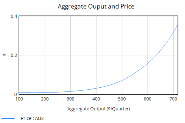
One simulation result that shows the relationship between the change in aggregate output and the inflation rate is the following:

Concluding remark

In this part of notebook, we articulate Keynes’s general theory of inflation. Keynes’s theory is nothing more than the cost of production approach to inflation, which goes back to Adam Smith and Karl Marx’s discussion in the history of economic thoughts. This cost of production theory of inflation is contrasted with the classical quantity of money theory of inflation, according to which the change in the quantity of money proportionately affects the price level. We learn that this classical inflation theory is based upon a series of underlying assumptions such as the full employment assumption and zero or negligible precautionary and speculative motives for holding money in the economy.

Many post-WWII American Keynesian economists have sought to find a reliable inflation modeling framework under constantly evolving macroeconomic and monetary circumstances in the U.S. Some of them reframed Keynes’s broader cost of production approaches to the price level and inflation rate into a narrowly defined relationship between the nominal wage rate and unemployment rate. This particular focus of the relationship between the two variables has been better known as the Phillips curve theory of inflation, or the Phillips curve debate.

We will reconstruct and examine the validity of the Phillips curve theory of inflation in a separate note. It will suffice to say for now that A.W. Phillips’s initial finding on the seemingly stable negative correlation between the change in nominal wage rates and unemployment rates observed from the British data was quickly embraced by Paul Samuelson and Robert Solow, then influential two American orthodox Keynesian economists. They reconstructed the similar Phillips curve for the U.S. economy and presented it as if it was an accurate representation of Keynes’s inflation theory as well as a practical policy guidance. Both Monetarists led by Milton Friedman and New Classical School led by Robert Lucas disputed the validity of this Phillips curve theory of inflation in the U.S., using their emphasis on rational economic agents’ inflation expectations.

A special case: Modeling the wage-price spiral dynamics

Introduction

One crucial contribution made by Keynes and his followers is their distinction between different states of the economy. The distinction between ‘less than full employment range’ and ‘the full employment level’ in the economy is the case in point. Depending on which state the economy is operating at, the policy goal of achieving the full employment via either the government’s fiscal policy or central bank’s monetary policy has a differential outcome.

This part of note introduces a few models that show the nonlinear inflation dynamics emerging from the ‘wage-price spiral’ domain. If the economic activity is stimulated too much at a given period moving beyond the full employment range, we can expect from Keynes’s cost of production approach to inflation that the so-called wage-price spiral phenomenon occurs. We can also anticipate that economic agents’ expectation about the future price and inflation can be formed and begin to play an important role in determining the actual inflation rate. The models presented below are an attempt to account for these phenomena.

Each section below is self-contained; each section introduces the core ideas of the respective model, explains how to set up and derives a relevant difference and/or differential equation, and how to find and visualize the solution. The last section concludes the scope and limitation of the respective model.

A simple wage-price interaction model

The core ideas, assumptions, and the model

Suppose that the nominal wage at time t , W(t), is increased by a constant rate (r) over the price level measured one period earlier, P(t-1). Workers are assumed to engage in a series of collective bargaining efforts to catch up with the rise in the past price level that has undermined their real purchasing power, the real wage (W/P). The producer, in turn, charges a markup (m) over the labor cost incurred in the previous production (W[t-1]).

Here, we temporarily ignore the effect of the change in the price of other factors of production such as the user cost of capital equipment and the price of intermediate goods and raw materials. How would these nominal wage and price setting behavior interact with one another as times goes by?

Given these assumptions, we can write down the following two first-order, linear, autonomous, and homogeneous difference equations that constitute the simple wage-price dynamic model.

W[t]=(1+r)*P[t-1]

(

)

P[t]=(1+m)*W[t-1]

(

)

Here, W(t) is the nominal wage level at time t, P[t] is the price level measured at the same time t. Both r and m are positive constants, which, respectively, represents the fixed growth rate of nominal wage that workers gain from a successful collective bargaining effort and a constant markup that the producer-seller of the product charges over the labor cost. Once again, we intentionally ignore non-labor cost in the production; we also ignore labor market variables that affect the wage bargaining practice and its effectiveness; finally, we assume that the firm-employer’s markup pricing ability stays constant.

The analytical solution

Using this ‘RSolve’ function, we can generate the following analytical solution to this system of two difference equations:

Clear[W,P,r,m,t];RSolve[{W[t]==(1+r)*P[t-1],P[t]==(1+m)*W[t-1],W[0]==W0,P[0]==P0},{W[t],P[t]},t]//Simplify

Out[]=

P[t]

P0

1+m

1+r

)

t/2

(1+m)

t/2

(1+r)

-

1+m



1+m

1+r

)

t/2

(1+m)

t/2

(1+r)

W0

1+r

,W[t]

1+r



1+m

1+r

)

t/2

(1+m)

t/2

(1+r)



1+m

+

1+m

1+r

)

t/2

(1+m)

t/2

(1+r)

W0

A static visualization with fixed parameters

To see how this set of solution functions behave, let us assign an arbitrary value to each of the two initial values and coefficients. Suppose that:

An observation

In this model, we can observe that the nominal wage increases as the price level rises. The increase in the nominal wage positively feedbacks on the firm’s markup pricing vice versa. How fast and how much the change in the price level is affected by the change in the nominal wage depends on the two parameter, r and m, which respectively represents the worker’s collective bargaining power and the producer’s ability to charge a markup price.

Frisch et al’s ‘wage-price spiral’ model

The core ideas and the model

Frisch, Haavelmo, Norregaard-Rasmussen and Zeuthen considered the following systems when they built a ‘wage-price spiral’ model of labor market and inflation (Sydsaeter et al 2008: 410):

In this formulation, Frisch et.al imposes the idea that the change in the price level at time t is a function of the change in the wage level at time t by a factor of β . The wage level at t+1 also depends on a fractional increase in the previous wage level at time t. When workers negotiate with their employers, they wish to compensate for the eroded real wage by considering the current price level by a factor of c. Together, the growth rate of wage at t+1 is set to be equal to the inflation rate at time t.

The analytical solution

By substituting the third equation (5) into the second-order difference equation, we get the following solution:

A static visualization with fixed parameters

One thing that is important in this model is that this system can be made globally asymptotically stable only when cβ is less than 1. Otherwise, the system will be explosive.

For example, suppose γ = 0.5, β = 1, and c = 1.5 with the two initial values W0=1 and W1=1.2. Then the solution of the system becomes W(t) diverges away from its steady state solution.

Suppose this time that γ = 0.5, β = 0.4, and c = 1.5, then the solution of W(t) converges to its steady state value.

An observation

This ‘wage-price spiral’ model is very insightful because it helps us better understand a certain real-world economic phenomena. The increase in either wage or price variable also increases in price and wage variable with some time delays, dynamically affecting their future behaviors. The two crucial parameters β and c, which respectively represents the firm’s markup pricing ability and the workers’ bargaining power to increase their diminished real wage determine the dynamic interaction between wage and price.

It is crucial to think about various options for stabilizing the inflationary pressure. In this model, it seems that there are only two choices available; either reducing workers’ collective bargaining power to stamp down the pressure for wage increase, or bring down the producer-employer’s ability to charge a higher price. Is there any other way to consider the effect of the change in production cost in multi-sector economy on the price level?

From a theoretical point of view, the wage-price spiral phenomenon is an exceptional case that may happen only when the economy is pushed beyond its full employment range by sustained expansionary fiscal and monetary policies. Therefore, we cannot generalize the implied policy options unique to this special case beyond its context.

Concluding remark

In this part of notebook, we have learned how we can build and solve systems of difference equations that are relevant to the analysis of the interaction between nominal wage and price level variables in the wage-price spiral domain.

Each model has its own merits and limitations. Identifying the core ideas and assumptions are equally important as technical aspects of the model presented in this note.

Reference

John M. Keynes, The General Theory of Employment, Money and Interest. New York: Prometheus Books, 1997 [1936].

Knut Sydsaeter, Peter Hammond, Arne Strom, Atle Seierstad, and Arne Strom, Further Mathematics for Economic Analysis. Harlow, UK: Pearson, 2008 (2nd edition).

CITE THIS NOTEBOOK

Introduction to dynamic economic models: dynamic inflation models III
by Hee-Young Shin
Wolfram Community, STAFF PICKS, December 18, 2025
https://community.wolfram.com/groups/-/m/t/3593660