In the late 90s, when famous quantum algorithms (especially Shor’s) were published, stared the race to build first quantum computer. In that proses occur many technological difficulties due to non obvious way how to represent quantum states, unstable nature of themself and complicated measurement process. One of challenges is to design quantum circuits that perform functions which are fast and simple.
Initialization
Initialization
Basic quantum circuits
Basic quantum circuits
Every function in quantum computation can be presented as unitary operator in Hilbert space. Let’s take basic boolean function of 3 variables: . The function operator is decomposed in terms of CCNOT gates as default. One of the corresponding circuits may look like:
f(x,y,z)x||y||z
In[]:=
sampleCircuit=QuantumCircuitOperator[{"Grover",x||y||z}];sampleCircuit["Diagram"]
Out[]=
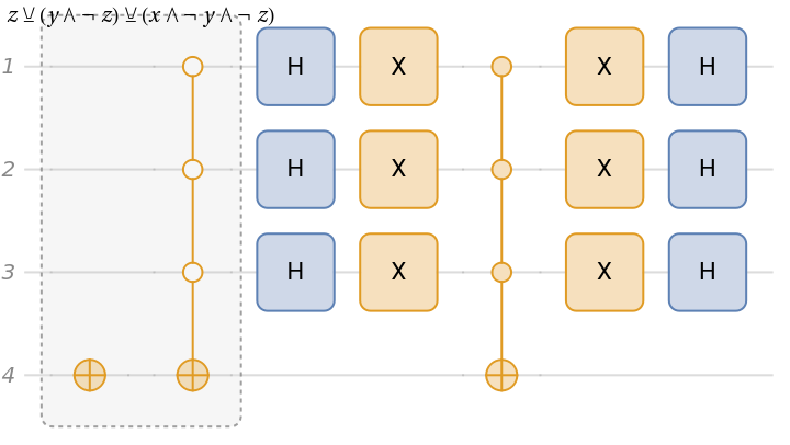
For measurements I used Grover’s algorithm circuit. It is more “quantum” way of using functions. That means, quantum computers wouldn’t be used for typical work as classical ones do it these days. They are more complicated and less efficient than current computers. Advantage of using quantum computers comes form specific algorithms which speed up some computations using quantum nature of things like entanglement. One of these algorithms is Grover’s algorithm. It transforms the Bell entangled state into some state which dot product with the solution state is given by:sinAs success I understand getting the solution state on the output.where N is dimension of Hilbert space, M - number of solutions and k is number of iterations of algorithm.To maximize this probability there is some of iterations required.
P
succ
2
(2k+1)arccos
1-
M
N
In[]:=
BarChart[QuantumPartialTrace[sampleCircuit[QuantumOperator["Z"->4]@QuantumState[{"UniformSuperposition",4}]],{4}]["Probability"],ChartLabels->Automatic]
Out[]=
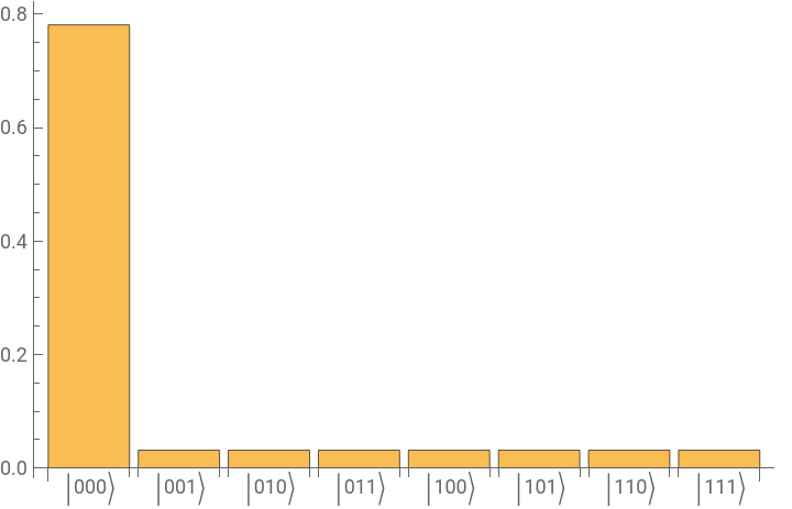
After first iteration, high probabilities doesn’t match the real solution. There is need to repeat the procedure.
Complexity
Complexity
There is no given way to measure complexity of quantum circuit similar to classical computation - time and memory complexity. We are forced to come up with some new way to measure how simple/fast/robust quantum circuit is. Let me introduce some metrics specific to boolean function.
Grover algorithm iterations number
Grover algorithm iterations number
Groover algorithm should be repeated until high probability of success will be achieved. This means that argument should be . There is a little chance that this will happen at integer value. That is the reason the 100% success is unlikely. Moreover this number depends only on dimension of solutions space (equivalently number of variables) and number of solution of the boolean function. That means the-same-number-of solutions functions can be treated as the same from the algorithm point of view. Because of that fact I consider only one representative of each class with different number of solutions.Here is an example of the best number of iterations for 14-variable function.
sin
π
2
In[]:=
Show[ListPlot[Table[argMaks[2^14,i],{i,1,69}],PlotLegends->{"The best < 100 number of iterations"},AxesLabel->{"Number of solutions"," The best iterations no."}],Plot[grovMax[2^14,q],{q,1,69},PlotStyle->{Gray,Opacity[0.7]},PlotLegends->{"Theoretical 100% success (non-inteer valued)"}]]
Out[]=
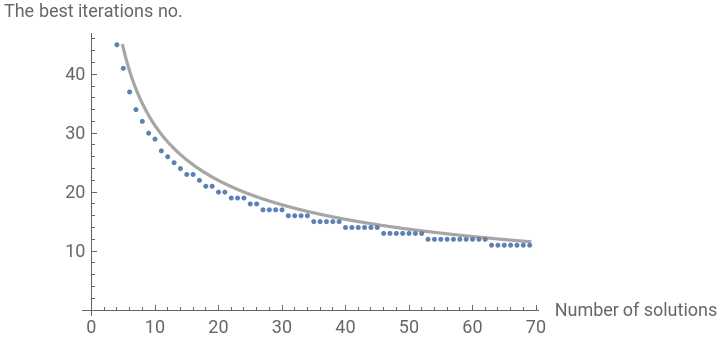


More iteration theoretically can improve probability of success, finding a maximum occurring closer to the integer-valued argument, however experimentally more complicated circuit increases noise influence.
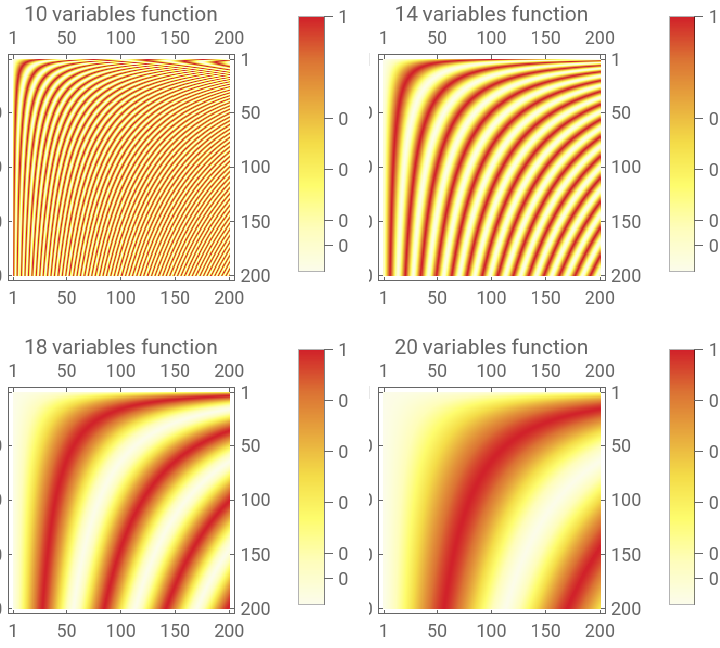
Undermentioned plots show the probability of success as function of number of solutions and number of iterations for a different number of variables function. As it springs from formula you can find multiple solutions, where probability is high (sin function periodicity) The first number of iterations with high success increases with number of variables and decreases with number of solutions.
Undermentioned plots show the probability of success as function of number of solutions and number of iterations for a different number of variables function. As it springs from formula you can find multiple solutions, where probability is high (sin function periodicity) The first number of iterations with high success increases with number of variables and decreases with number of solutions.
In[]:=
GraphicsGrid[ArrayReshape[Table[MatrixPlot[Table[grovTab[2^j,i,200],{i,1,200}],ColorFunction->"TemperatureMap",PlotLegends->Automatic,AxesLabel->Automatic,PlotLabel->StringForm["`1` variables function",j]],{j,{10,14,18,20}}],{2,2}]]
Out[]=
Robustness
Robustness
In every real circuit occurs some undesirable effects which causes changes of qubit states. This phenomenon is called noise. I performed simulations of circuit with bit flip effect happening just before the measurement.
In[]:=
sampleCircuitWithNoise=QuantumCircuitOperator[Insert[sampleCircuit["Operators"],QuantumChannel[{"BitFlip",p},Range[4]],2]];sampleCircuitWithNoise["Diagram"]
Out[]=
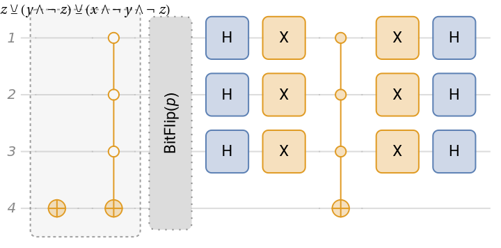
Undermentioned plot shows the results of simulations of measuring the probability of success of 5-variables function with various number of solutions and bit-flip probability. The dashed green line show the theoretical probability from Grover’s algorithm formula.
In[]:=
Manipulate[Show[Plot[groverSuccess[2^5,i,k-1],{k,1,20},PlotStyle->{Green,Dashed,Opacity[0.4]},PlotRange->{{0,20},{0,1}},PlotLabel->StringForm["Bitflip Probability `1`",Range[0,1,0.1][[j]]]],ListPlot[bool5[[i]][[j]],PlotStyle->Red,PlotRange->{Automatic,{0,1}}],AxesLabel->{"Number of iterations"," Probability of success"}],{{i,5,"Number of solutions"},1,13,1},{{j,5,"Bit-flip probability"},1,11,1},SaveDefinitions->True]
Out[]=


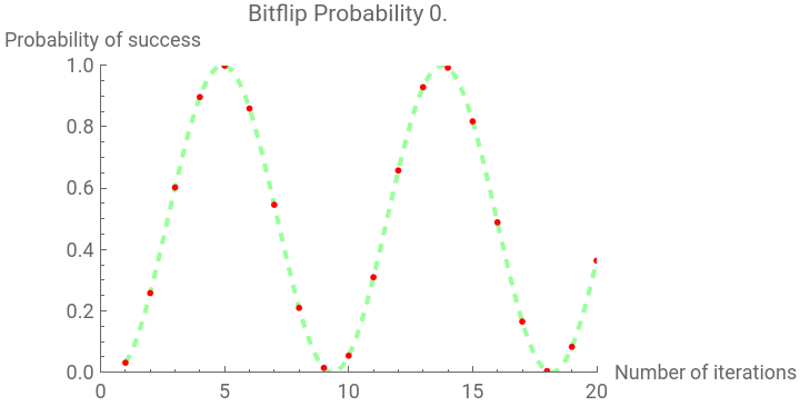
You can see that theoretical predictions match the simulation results in the zero bit-flip probability case.
Probability of success for functions with 1-4 solutions, parametrized by bit-flip propability.
In[]:=
Manipulate[ListLinePlot[Map[Part[#,i]&,Take[bool5,4]],PlotRange->{Automatic,{0,1}},PlotStyle->{Opacity[0.3]},PlotLegends->Range[7],PlotLabel->StringForm["Bitflip Propability `1`",Range[0,1,0.1][[i]]],InterpolationOrder->3,AxesLabel->{"Number of iterations"," Propability of success"}],{{i,3,"Bit-flip porpability"},1,11,1},SaveDefinitions->True]
Probability of success increases with number of solutions.
The same probability for the first functions with given number of solutions in range 1-13. Manipulate track-bar increases probability of bit-flip. Increasing trend is noticeable.
Noise in front of oracle
Noise in front of oracle
The most realistic noise substitute should be performed as noise quantum channel for every gate in circuit. However computations are very heavy and I simplified noise as operation before or after oracle.
In that way of simulating noise you can see it impacts on results less than noise behind oracle. The undermined plot shows comparison between them.
Plain lines shows the front noise functions, dashed - end.
Again the maximum success probability as function of bit-flip probability and number of solutions:
Again the maximum success probability as function of bit-flip probability and number of solutions:
You can see that circuit with noise at the beginning is significantly better, especially with functions with smaller number of solutions.
Acknowledgments
Acknowledgments
I would like to thank all the International Physicist’s Tournament 2023 participants for unforgettable experience, especially Poland team form University of Warsaw, I’m there thanks to you. I want to thanks my mentors Mano and Nik for help and dedicated time. Thank you, Mads for help and care about my project. Thank you all WSS2023 participants for a great time.
Literature
Literature
CITE THIS NOTEBOOK
CITE THIS NOTEBOOK
Quantum gate complexity of Boolean functions
by Jakub Grabarczyk
Wolfram Community, STAFF PICKS, July 13, 2023
https://community.wolfram.com/groups/-/m/t/2959886
by Jakub Grabarczyk
Wolfram Community, STAFF PICKS, July 13, 2023
https://community.wolfram.com/groups/-/m/t/2959886