This article presents an exploration into the application of ordinary differential equations in modeling physical phenomena, specifically harmonic oscillator motion. Additionally, it investigates the role of metamathematics in understanding the implications of these mathematical models. The article illuminates how software tools like Mathematica can assist in solving and visualizing these equations, contributing to a deeper comprehension of the mathematical structures and their physical significance.
Introduction
Introduction
Ordinary differential equations play a pivotal role in mathematics and their application in physical sciences . In particular, models like the motion of harmonic oscillators can be encapsulated by such equations . A simple illustration of this idea is the harmonic oscillator equation :
2
d
d
2
t
2
ω
This equation describes the motion of a harmonic oscillator (like a spring or a pendulum) with a constant . The general solution to this equation is :
2
ω
x(t)Acos(ωt)+Bsin(ωt)
The constants A and B are determined by the initial conditions of the motion .
Metamathematics and its implications
Metamathematics and its implications
The approach of metamathematics is the investigation into the deeper semantic and philosophical questions that arise from mathematics and their application . For example, a metamathematical question for the above equation could be : "What does it mean for this to be the 'solution' to the differential equation?" or "What does this solution tell us about the nature of the oscillator's motion?" or even "How can we be certain that this solution is 'correct'?" . These questions can lead to deeper analyses concerning the nature of mathematics and their application to the physical world .
Use of Mathematica in understanding mathematical models
Use of Mathematica in understanding mathematical models
With the aid of software like Mathematica, we can solve and graphically depict these kinds of equations . The harmonic oscillator equation, for example, can be solved using the `DSolve` command and graphically represented using the `Plot` command . These computational techniques allow for a direct investigation into the consequences of the mathematical models and an understanding of the physical significance of the solutions .
Real-world examples
Real-world examples
◼
Simple Harmonic Oscillator (e.g., Mass-Spring System)
In[]:=
solution=DSolve[{x''[t]+ω^2*x[t]==0,x[0]==x0,x'[0]==v0},x[t],t]
Out[]=
x[t]
x0ωCos[tω]+v0Sin[tω]
ω
In[]:=
Plot[Evaluate[x[t]/.solution/.{ω->2*Pi,x0->1,v0->0}],{t,0,10},PlotLabel->"Mass-Spring System"]
Out[]=
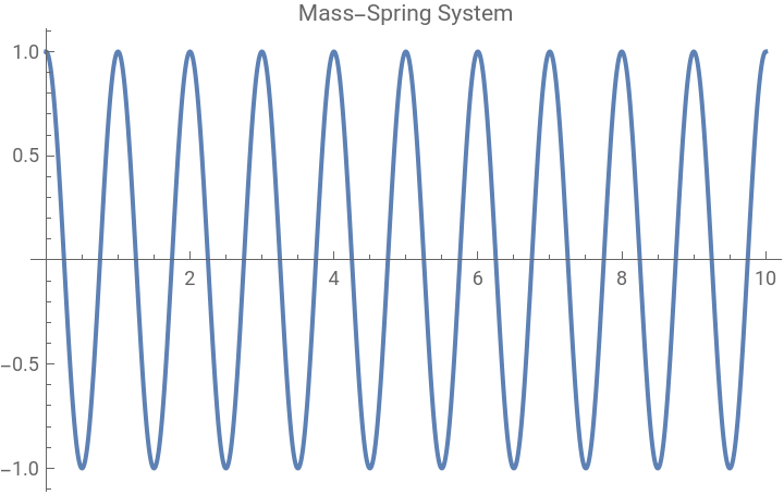
Here we assume that the mass is displaced by 1 meter initially and released from rest . The natural frequency of oscillation is rad/sec.
(ω)
2π
◼
Damped Oscillator (e.g., Car Suspension)
In[]:=
solution=DSolve[{x''[t]+γ*x'[t]+ω^2*x[t]==0,x[0]==x0,x'[0]==v0},x[t],t]
Out[]=
x[t]-2t-γ--4v0+2t-γ+-4v0-t-γ--4x0γ+t-γ+-4x0γ+t-γ--4x0-4+t-γ+-4x0-4
1
2-4
2
γ
2
ω
1
2
2
γ
2
ω
1
2
2
γ
2
ω
1
2
2
γ
2
ω
1
2
2
γ
2
ω
1
2
2
γ
2
ω
2
γ
2
ω
1
2
2
γ
2
ω
2
γ
2
ω
In[]:=
Plot[Evaluate[x[t]/.solution/.{ω->2*Pi,γ->1,x0->1,v0->0}],{t,0,10},PlotLabel->"Car Suspension"]
Out[]=
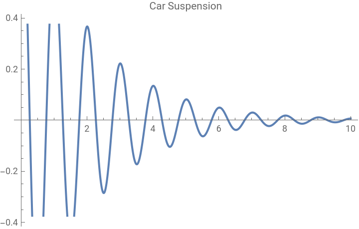
Here the car suspension is compressed by 1 meter initially and released from rest . The natural frequency of oscillation is rad/sec and the damping factor is 1.
(ω)
2π
(γ)
◼
Driven Oscillator (e.g., Electric Circuit with Alternating Current)
In[]:=
solution=DSolve[{x''[t]+γ*x'[t]+ω^2*x[t]==F0*Cos[ω1*t],x[0]==x0,x'[0]==v0},x[t],t]
Out[]=
x[t]t-γ--4F0γ-t-γ+-4F0γ-2t-γ--4v0+2t-γ+-4v0-t-γ--4x0γ+t-γ+-4x0γ-t-γ--4F0-4-t-γ+-4F0-4+t-γ--4x0-4+t-γ+-4x0-4+t-γ--4F0γ-t-γ+-4F0γ-2t-γ--4v0+2t-γ+-4v0-t-γ--4x0+t-γ+-4x0+4t-γ--4v0-4t-γ+-4v0+2t-γ--4x0γ-2t-γ+-4x0γ+t-γ--4F0-4+t-γ+-4F0-4+t-γ--4x0-4+t-γ+-4x0-4-2t-γ--4x0-4-2t-γ+-4x0-4-2t-γ--4v0+2t-γ+-4v0-t-γ--4x0γ+t-γ+-4x0γ+t-γ--4x0-4+t-γ+-4x0-4+2F0-4Cos[tω1]-2F0-4Cos[tω1]+2F0γ-4ω1Sin[tω1]2-4(+-2+)
1
2
2
γ
2
ω
2
ω
1
2
2
γ
2
ω
2
ω
1
2
2
γ
2
ω
4
ω
1
2
2
γ
2
ω
4
ω
1
2
2
γ
2
ω
4
ω
1
2
2
γ
2
ω
4
ω
1
2
2
γ
2
ω
2
ω
2
γ
2
ω
1
2
2
γ
2
ω
2
ω
2
γ
2
ω
1
2
2
γ
2
ω
4
ω
2
γ
2
ω
1
2
2
γ
2
ω
4
ω
2
γ
2
ω
1
2
2
γ
2
ω
2
ω1
1
2
2
γ
2
ω
2
ω1
1
2
2
γ
2
ω
2
γ
2
ω1
1
2
2
γ
2
ω
2
γ
2
ω1
1
2
2
γ
2
ω
3
γ
2
ω1
1
2
2
γ
2
ω
3
γ
2
ω1
1
2
2
γ
2
ω
2
ω
2
ω1
1
2
2
γ
2
ω
2
ω
2
ω1
1
2
2
γ
2
ω
2
ω
2
ω1
1
2
2
γ
2
ω
2
ω
2
ω1
1
2
2
γ
2
ω
2
γ
2
ω
2
ω1
1
2
2
γ
2
ω
2
γ
2
ω
2
ω1
1
2
2
γ
2
ω
2
γ
2
γ
2
ω
2
ω1
1
2
2
γ
2
ω
2
γ
2
γ
2
ω
2
ω1
1
2
2
γ
2
ω
2
ω
2
γ
2
ω
2
ω1
1
2
2
γ
2
ω
2
ω
2
γ
2
ω
2
ω1
1
2
2
γ
2
ω
4
ω1
1
2
2
γ
2
ω
4
ω1
1
2
2
γ
2
ω
4
ω1
1
2
2
γ
2
ω
4
ω1
1
2
2
γ
2
ω
2
γ
2
ω
4
ω1
1
2
2
γ
2
ω
2
γ
2
ω
4
ω1
2
ω
2
γ
2
ω
2
γ
2
ω
2
ω1
2
γ
2
ω
2
γ
2
ω
4
ω
2
γ
2
ω1
2
ω
2
ω1
4
ω1
In[]:=
Plot[Evaluate[x[t]/.solution/.{ω->2*Pi,γ->0.5,F0->2,ω1->2*Pi,x0->0,v0->0}],{t,0,10},PlotLabel->"AC Circuit"]
Out[]=
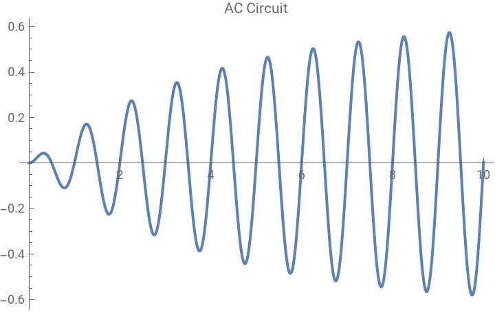
Here the circuit has a natural frequency of rad/sec, damping factor of 0.5, and it is driven by an alternating current with amplitude 2 and frequency rad/sec .
2π
2π
Conclusion
Conclusion
Thus, metamathematics provides a framework for examining the deep issues that arise from the application of mathematics to the physical sciences while simultaneously acknowledging the complexity and dynamism of the mathematical structures used to describe the physical world .
CITE THIS NOTEBOOK
CITE THIS NOTEBOOK
Metamathematics, Ordinary Differential Equations,and their Application to Harmonic Oscillator Motion
by Athanasios Paraskevopoulos
Wolfram Community, STAFF PICKS, August 4, 2023
https://community.wolfram.com/groups/-/m/t/2983518
by Athanasios Paraskevopoulos
Wolfram Community, STAFF PICKS, August 4, 2023
https://community.wolfram.com/groups/-/m/t/2983518