Jackiw-Rebbi states: Numerical Solutions
Jackiw-Rebbi states: Numerical Solutions
In this notebook we want to find the Jacki-Rebbi states, which are solutions for a Dirac Hamiltonian with a mass that changes sign as x goes from negative to positive, i.e. sign[m(x)] = sign[x].
This problems has an analytical solution (see [1]). However, in this notebook these are only found then |m(x)|=|m(-x)|. I would appreciate any help/suggestion that might be useful to find the solutions when |m(x)|≠|m(-x)|.
This problems has an analytical solution (see [1]). However, in this notebook these are only found then |m(x)|=|m(-x)|. I would appreciate any help/suggestion that might be useful to find the solutions when |m(x)|≠|m(-x)|.
Introduction
Introduction
Theoretical Approach
Theoretical Approach
Here we want to obtain numerical solutions for Jackiw-Rebbi states. These states are found when we have a massive Dirac Hamiltonian in 1D with a finite negative mass for x<0 and a positive mass for x>0. The Dirac Hamiltonian is
h(k) = v ℏ k + =
where m =
.
σ
x
2
mv
σ
z
m | -ivℏ ∂ x |
-ivℏ ∂ x | -m |
|
This Hamiltonian acts on a state and we obtain the following system of PDE
ψ(x)=
T
(,)
ψ
1
ψ
2
2
mv
ψ
1
-ivℏ
∂
x
ψ
2
ψ
1
-
2
mv
ψ
2
-ivℏ
∂
x
ψ
1
ψ
2
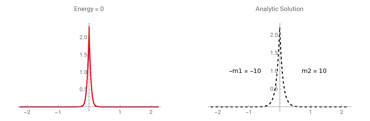
In this notebook we use ℏ = v = 1. The analytics solutions for the zero-energy bound states are known (see [1], for example), and are:
ψ(x) =+ .
1/2
m
1
m
2
m
1
m
2
1 |
i |
-|m(x)x|
e
Numerical Solution
Numerical Solution
Parameters
Parameters
Domain of the problem
Domain of the problem
Since we are looking for bound-states (edge-states at the domain wall) we expect our solutions to decay exponentially. Therefore, we compute the length (domain of study) of the problem using , where p is defined by .
l=
p-log(√m)
m
ψ(x=L)=
-p
10
In[]:=
p=20;(*Lengthoftheproblem*)l=(p+Log[Min[Abs@{m1,m2}]])/Min[Abs@{m1,m2}]//N
Out[]=
20.+Log[Min[Abs[m1],Abs[m2]]]
Min[Abs[m1],Abs[m2]]
Mass function
Mass function
In[]:=
(*Masses*)m1=10;m2=10;(*Massfunction*)mass1d[m1_,m2_,x_]:=m2UnitStep[x]-m1UnitStep[-x];Plot[mass1d[m1,m2,x],{x,-10,10}]
Out[]=
Solutions
Solutions
To solve this problem we use the FEM method NDEigensytem.
Solve
Solve
Expected energy. NDEigensystem gives the solutions with the lowest absolute values. If we want to find solutions with energy ϵ, we need to “translate” our new 0 to this value.
In[]:=
(*Expectedenergy*)ϵ=0;(*numberofsolutions*)nSols=10;
Numerical solver
In[]:=
{vals,sols}=NDEigensystem[{(*DiracEquation*)-Iud'[x]+(mass1d[m1,m2,x]-ϵ)*uu[x],-Iuu'[x]+(-mass1d[m1,m2,x]-ϵ)*ud[x],(*Boundaryconditions*)DirichletCondition[uu[x]0,True],DirichletCondition[ud[x]0,True]},{uu[x],ud[x]},{x,-l,l},nSols];

Results
Results
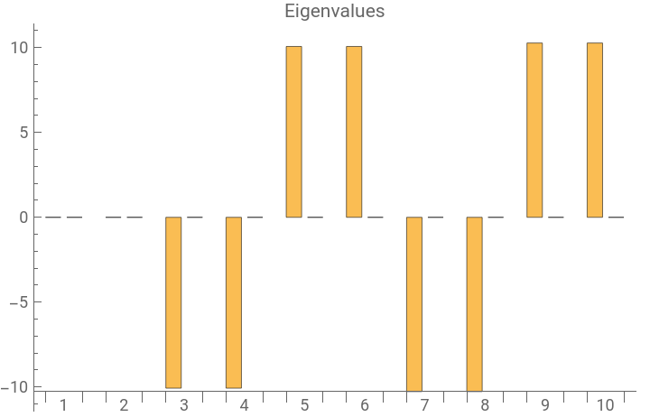
Eigenvalues (let’s look for zero-energies)
In[]:=
vals//Chop
Out[]=
{0,0,-10.0686,-10.0686,10.0686,10.0686,-10.2716,-10.2716,10.2716,10.2716}
Plot to visualize energies
In[]:=
BarChart[ReIm/@vals,ChartLegends{"Real Part","Imaginary Part"},ChartLabels{Range[nSols],None},PlotLabel"Eigenvalues",ImageSizeMedium]
Out[]=


Let’s find the normalization constants
In[]:=
normConst=Total/@(Sqrt@Partition[NIntegrate[Abs[#]^2/.xx0,{x0,-l,l}]&/@Flatten[sols],2]);solsNormalized=sols/normConst;
15
10
11
10
15
10
11
10
Let’s plot the solutions
In[]:=
sol=1;GraphicsGrid[{{Plot[Abs[solsNormalized[[sol]]]^2/.{xx0}//Evaluate,{x0,-l,l},PlotRangeAll,PlotLabelStringJoin["Energy = ",ToString[vals[[sol]]//Chop//Re]],PlotStyle{Blue,Red},ImageSizeMedium],Plot[Sqrt[m1m2/(m1+m2)]Exp[-Abs[mass1d[m1,m2,x]x]],{x,-l,l},PlotLabel"Analytic Solution",PlotRangeAll,PlotStyle{Dashed,Black},Epilog{Text[StringJoin["-m1 = -",ToString@m1],{-l/2,1}],Text[StringJoin["m2 = ",ToString@m2],{l/2,1}]},ImageSizeMedium]}}]
Out[]=
◼
Solutions where the energy is greater than the mass are not meaningful.
Problem with different mass
Problem with different mass
When I use different masses I am not able to obtain the solutions. For example, using -m1 and 2m1
Different mass function
Different mass function
Solutions
Solutions
To solve this problem we use the FEM method NDEigensytem.
Expected energy. NDEigensystem gives the solutions with the lowest absolute values. If we want to find solutions with energy ϵ, we need to “translate” our new 0 to this value.
Numerical solver
Results
Results
Eigenvalues (let’s look for zero-energies)
Plot to visualize energies
Let’s find the normalization constants
Let’s plot the solutions
◼
I’ll appreciate any advice that can improve this in order to obtain solutions for different mass values.
References
References
[1] Shen, S. Q. (2012). Topological insulators (Vol. 174). Berlin: Springer.