On 29 February 2020, the China National Health Commission reported 423 new cases of coronavirus for Hubei and only 4 cases for the rest of the country. The logistic function fit to the data from the Johns Hopkins CSSE, have been showing for a while that the epidemic should end outside of the Hubei province in the first week of March. The recent report seems to confirm this prediction.
This notebook contains some updated and new functions that were not in my previous posts.
This notebook contains some updated and new functions that were not in my previous posts.
Data Source
Data Source
The latest data gets updated on dashboard above before it is loaded to GitHub, which is the source for the notebook.
Procedures
Procedures
In[]:=
Clear[modelFitDisplay];modelFitDisplay[NLM_,data_,opts___]:=Module[{bands,p0,p1},bands[t_]=NLM["SinglePredictionBands",ConfidenceLevel0.95];p0=Plot[{NLM[t],bands[t]},{t,1,data[[-1]][[1]]+5},opts,Filling{2{1}},PlotStyle{Darker@Red,Darker@Orange,Darker@Orange},GridLinesAutomatic,PlotRangeAll,opts];p1=ListPlot[Tooltip[#,#]&/@data,PlotRangeAll];Show[p0,p1]];
In[]:=
Clear[derivativeDisplay];derivativeDisplay[NLM_,data_,opts___]:=Module[{daynum,end,peak},daynum=data[[-1]][[1]];peak=t0/.NLM["BestFitParameters"];end=x/.FindRoot[NLM'[x]1,{x,peak,peak+200},(*forcetorighttail*)Method"Brent"][[1]];Print["Last case: ",DateString[DatePlus[{2020,1,21},Ceiling@end],"DateShort"]];Show[Plot[{NLM'[x],NLM''[x]},{x,data[[1]][[1]]-4,daynum+5},opts,GridLinesAutomatic,PlotRangeAll,PlotLegends{"First Derivative","Second Derivative"}],ListPlot[Tooltip[#,#]&/@{{daynum,NLM'[daynum]}},PlotStyle{Red,PointSize[0.02]}]]];
In[]:=
Clear[dataD1];dataD1[data_,{k_,L_}]:=Table[{data[[i]][[1]],kdata[[i]][[2]](1-data[[i]][[2]]/L)},{i,Length[data]}];
In[]:=
logistic=L/(1+Exp[-k(t-t0)]);
In[]:=
Clear[logisticDEFit];logisticDEFit[data_,graphic_:True,optsInterpolation___]:=Module{dataFn,dataDE,dataDEPlot,deModel,deNLM,bands},dataFn=Interpolation[data,optsInterpolation,Method"Spline"];dataDE={dataFn[#],dataFn'[#]}&/@data[[All,1]];dataDEPlot=ListPlot[dataDE,PlotStyleDarker@Red,GridLinesAutomatic,PlotRangeAll];deModel=kx1-;deNLM=NonlinearModelFit[dataDE,deModel,{k,L},x];If[graphic,bands[L_]=deNLM["SinglePredictionBands",ConfidenceLevel0.95];Print@Show[Plot[{deNLM[x],bands[x]},{x,0,L/.deNLM@"BestFitParameters"},GridLinesAutomatic,Filling{2->{1}},FrameTrue,FrameLabel{"Cases","New Cases Per Day"},PlotRangeAll,PlotLabel"Logistic Differential Equation"],dataDEPlot]];Flatten@{deNLM@"BestFitParameters",FindRoot[dataFn[t0]L/2/.deNLM["BestFitParameters"],{t0,data[[-1]][[1]]}]};
x
L
Import Data
Import Data
In[]:=
deaths=Import["https://raw.githubusercontent.com/CSSEGISandData/COVID-19/master/csse_covid_19_data/csse_covid_19_time_series/time_series_19-covid-Deaths.csv"];deaths[[1]][[-1]]
Out[]=
2/28/20
In[]:=
deathData=AssociationThread[First@deaths,#]&/@Rest[deaths]//Dataset;
In[]:=
confirmed=Import["https://raw.githubusercontent.com/CSSEGISandData/COVID-19/master/csse_covid_19_data/csse_covid_19_time_series/time_series_19-covid-Confirmed.csv"];confirmed[[1]][[-1]]
Out[]=
2/28/20
Setup Datasets
Setup Datasets
In[]:=
caseData=AssociationThread[First@confirmed,#]&/@Rest[confirmed]//Dataset;
In[]:=
chinaCaseData=caseData@Select[#"Country/Region""Mainland China"&];chinaDeathData=deathData@Select[#"Country/Region""Mainland China"&];
In[]:=
keys=Keys[First@Normal@caseData];Keys[First@Normal@deathData];
In[]:=
deathCases=Transpose[{Range[Length@keys-4],Values@Normal[chinaDeathData[Total,Drop[keys,4]]]}];confirmedCases=Transpose[{Range[Length@keys-4],Values@Normal[chinaCaseData[Total,Drop[keys,4]]]}];
In[]:=
notHubeiData=chinaCaseData@Select[#"Province/State"≠"Hubei"&];notHubeiCases=Transpose[{Range[Length@keys-4],Values@Normal[notHubeiData[Total,Drop[keys,4]]]}];
In[]:=
hubeiData=chinaCaseData@Select[#"Province/State""Hubei"&];hubeiCases=Transpose[{Range[Length@keys-4],Values@Normal[hubeiData[All,Drop[keys,4]]][[1]]}];
China Death Data
China Death Data
In[]:=
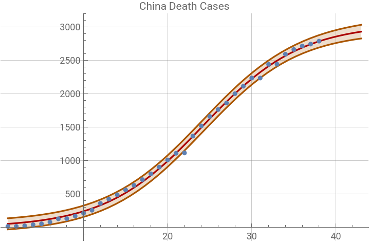
deathsNLM=NonlinearModelFit[deathCases,logistic,{{k,0.3},{L,3000},{t0,25}},t];deathsNLM@"BestFitParameters"
Out[]=
{k0.172041,L3044.88,t024.2041}
Out[]=
In[]:=
deathsNLM@"ParameterConfidenceIntervalTable"
Out[]=
Estimate | Standard Error | Confidence Interval | |
k | 0.172041 | 0.00394588 | {0.16403,0.180052} |
L | 3044.88 | 41.6121 | {2960.4,3129.36} |
t0 | 24.2041 | 0.226153 | {23.745,24.6632} |
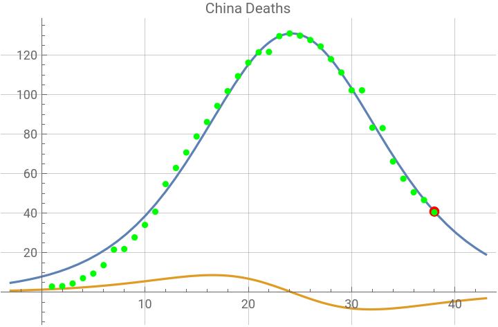
The graphic below shows the first and second derivative plots of the logistic function. The red dot is at the current day number on the first derivative curve. The green dots are the points calculated by the logistic differential equation, using each data point. The prediction for the last case date is printed (probably not accurate until there are at least three weeks of new data).
Last case: Sun 22 Mar 2020
Out[]=


China Clinical Cases
China Clinical Cases
In[]:=
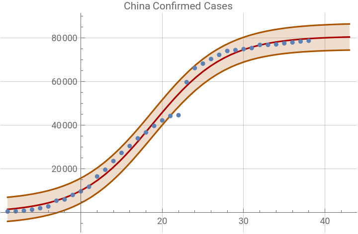
casesNLM=NonlinearModelFit[confirmedCases,logistic,{{k,0.3},{L,80000},{t0,25}},t];casesNLM@"BestFitParameters"
Out[]=
{k0.221968,L80902.5,t018.7671}
Out[]=
China Cases Outside Hubei
China Cases Outside Hubei
China Hubei Cases
China Hubei Cases
Fitting to the Logistic Differential Equation
Fitting to the Logistic Differential Equation
These graphics show a method of fitting to the equation for the logistic first derivative.
The value of x is the number of cumulative cases. This is a quadratic equation with roots at x = 0 and x = L, and peak at x = L/2. The first derivative is obtained from the data by making an interpolation function (Method “Spline” is default) from the data then using the function to calculate first derivative at each point. The 95% confidence intervals are shown for the quadratic fit. Clearly the data sets show quite a lot of irregularity by this method. The smoother data set, notHubei, shows the later points becoming more accurate. The parameters are similar to the fit to the logistic function.