Apply cellular automata (CA) rules to nested binary quasicrystal (QC) grids, categorize the dynamic pattern of the binary heat map, with various initial conditions and CA rules . We expect to see particle like excitations in certain cases. Start with a 1D QC, the Fibonacci, then expand to 2D Penrose tiling that is a network of the 1D QCs . So far we got some interesting result in both cases using the nearest neighborhood configurations and the binary on/off value conditions. Next we will consider more than just the nearest neighbors and also more complicated patch associated rules and also the nonlocal behaviors. For related research and interest, we will lift the quasicrystal up to higher dimension to visualize the dynamics from a different angle . Fourier transform will also be applied to the heat map to see the dynamics of the phase information .
CA in 1D Fibonacci chain, considering only the nearest neighbors (NB)
CA in 1D Fibonacci chain, considering only the nearest neighbors (NB)
In a Fibonacci chain (a 1D quasicrystal that consists of L and S segments in an aperiodic order), there are only 32 valued (binary on/off)nearest neighbor configurations, as shown in the below table in section 1. CA rules can be described by selecting certain cases to be on and off. A right combination of the on cases can give CA rules that describe left/right propagation, or other dynamics. Unlike conventional CA, the rules here also consider the different neighborhood of the quasicrystal, the L and S configurations.
Subsection 0 Chain generator
Subsection 0 Chain generator
Fibonacci chain function definition
In[]:=
FiChainGenerator[n_,s_,l_]:=Table[If[2+Floor[iGoldenRatio]-Floor[(i+1)GoldenRatio]0,l,s],{i,Fibonacci[n+1]}]
pplist1=Table[Total[FiChain1[[1;;i]]],{i,1,Length[FiChain1]}];pplist1=Prepend[pplist1,0];pplist1Plot=Table[{pplist1[[i]],-1},{i,1,Length[pplist1]}];
Chain1V=RandomChoice[{0,1},Length[FiChain1]];
In[]:=
Show[Table[Graphics[{Thickness0.005,If[(FiChain1[[i]]>1.5)&&(Chain1V[[i]]1),Red,If[(FiChain1[[i]]<1.5)&&(Chain1V[[i]]1),Blue,Gray]],Line[{pplist1Plot[[i]],pplist1Plot[[i+1]]}]}],{i,1,50-1}],Table[Graphics[{PointSize[0.005],Black,Point[pplist1Plot[[i]]]}],{i,1,50}]]
Out[]=
Nearest neighbor configuration and the CA rules
Nearest neighbor configuration and the CA rules
Based on the 32 nearest neighbor configurations, 11 CA rules are explored on 3 different initial conditions.
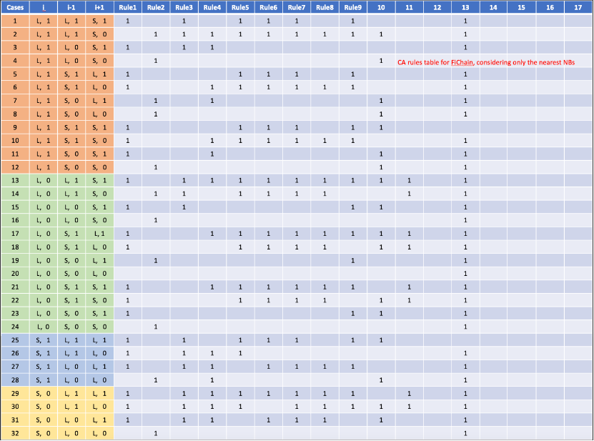
CA rule definitions
CA rule definitions
Choices of initial conditions
Choices of initial conditions
ARandomon/offmapontheFibonaccichainInitialCondition1={1,0,0,1,1,1,0,1,0,1,1,0,1,0,1,1,1,0,0,1,1,0,1,1,0,1,0,0,0,0,1,1,1,0,0,0,0,1,0,0,1,1,1,0,1,1,1,1,1,0,1,0,0,0,0,1,0,0,0,0,1,1,1,1,1,0,0,0,0,1,0,0,0,0,0,0,0,1,0,0,1,1,0,1,1,0,0,0,0,0,1,1,0,1,1,0,1,1,1,1,0,1,0,1,1,0,0,0,0,1,1,0,1,0,0,0,1,1,1,0,0,0,1,0,1,0,0,0,0,1,0,1,1,0,1,1,0,0,1,1,0,1,0,1,1,0,0,1,0,1,1,0,0,1,1,1,1,0,1,1,0,1,0,0,0,1,1,1,0,1,0,1,1,1,1,0,0,1,0,1,0,1,0,0,0,0,0,0,1,0,1,0,0,1,0,1,1,1,1,0,1,1,1,1,0,1,1,0,0,0,0,1,1,1,1,0,1,0,1,0,1,1,1,1,0,1,1,1,1,0,1,1,1,0,0,0,0,0,0,1,1,1,0,1,0,1,0,0,1,0,1,1,1,1,0,0,1,1,1,1,1,1,0,0,1,1,1,0,1,1,0,1,0,0,1,0,0,0,0,0,1,1,0,1,1,0,1,1,0,0,0,1,1,0,0,1,0,1,0,0,0,0,0,0,1,1,1,0,0,0,1,1,1,1,1,0,1,0,0,0,1,1,1,0,1,1,0,1,1,1,1,0,0,1,0,0,1,1,0,0,0,1,0,0,0,1,1,1,0,0,0,1,1,0,0,0,0,0,1,1,0,1,0,1,1,1,1,1,1,1,0,1,0,1,1,1};
ApalindromesectionontheFibonaccichainInitialCondition2={0,0,0,0,0,0,0,0,0,0,0,0,0,0,0,0,0,0,0,0,0,0,0,0,0,0,0,0,0,0,0,0,0,0,0,0,0,0,0,0,0,0,0,0,0,0,0,0,0,0,0,0,0,0,0,0,0,0,0,0,0,0,0,0,0,0,0,0,0,0,0,0,0,0,0,0,0,0,1,1,1,1,1,1,1,1,1,1,1,1,1,1,1,0,0,0,0,0,0,0,0,0,0,0,0,0,0,0,0,0,0,0,0,0,0,0,0,0,0,0,0,0,0,0,0,0,0,0,0,0,0,0,0,0,0,0,0,0,0,0,0,0,0,0,0,0,0,0,0,0,0,0,0,0,0,0,0,0,0,0,0,0,0,0,0,0,0,0,0,0,0,0,0,0,0,0,0,0,0,0,0,0,0,0,0,0,0,0,0,0,0,0,0,0,0,0,0,0,0,0};
Alength13Fibonacci(usingsubstitutionrules)sectionontheFibonaccichainInitialCondition3={0,0,0,0,0,0,0,0,0,0,0,0,0,0,0,0,0,0,0,0,0,0,0,0,0,0,0,0,0,0,0,0,0,0,0,0,0,0,0,0,0,0,0,0,0,0,0,1,1,1,1,1,1,1,1,1,1,1,1,1,0,0,0,0,0,0,0,0,0,0,0,0,0,0,0,0,0,0,0,0,0,0,0,0,0,0,0,0,0,0,0,0,0,0,0,0,0,0,0,0,0,0,0,0,0,0,0,0,0,0,0,0,0,0,0,0,0,0,0,0,0,0,0,0,0,0,0,0,0,0,0,0,0,0,0,0,0,0,0,0,0,0,0,0,0,0,0,0,0,0,0,0,0,0,0,0,0,0,0,0,0,0,0,0,0,0,0,0,0,0,0,0,0,0,0,0,0,0,0,0,0,0,0,0,0,0,0,0,0,0,0,0,0,0,0,0,0,0,0,0};
Subsection 3 CA dynamic results
Subsection 3 CA dynamic results
Chain1V1=InitialCondition2(*Changeaccordinglyforeachdifferentinitialcondition*);
Chain1VList={Chain1V1};AbsoluteTiming[For[i=1,i≤30,i++,PList=Range[Length[Chain1VList[[i]]]];POn=Flatten[1+Position[PList[[2;;Length[PList]-1]],_?(Case13[Chain1VList[[i]],#]||Case14[Chain1VList[[i]],#]||Case17[Chain1VList[[i]],#]||Case18[Chain1VList[[i]],#]||Case21[Chain1VList[[i]],#]||Case22[Chain1VList[[i]],#]||Case29[Chain1VList[[i]],#]||Case30[Chain1VList[[i]],#]&),{1},HeadsFalse],1];(*Changeaccordinglyinsideoftheparenthethissforeachdifferentrule*)POff=Complement[PList,POn];Chain1Vi=Table[0,Length[Chain1VList[[i]]]];Chain1Vi[[POn]]=1;Chain1Vi[[POff]]=0;AppendTo[Chain1VList,Chain1Vi]]]
In[]:=
Manipulate[Graphics[{Join[Table[{If[(FiChain1[[ii]]>1.5)&&(Chain1VList[[i,ii]]1),Red,If[(FiChain1[[ii]]<1.5)&&(Chain1VList[[i,ii]]1),Blue,Gray]],Rectangle[{pplist1Plot[[ii,1]],1.5},{pplist1Plot[[ii+1,1]],-3.0}]},{ii,1,200-1}],Table[{PointSize[0.001],Black,Point[pplist1Plot[[i]]]},{i,1,200}]]},ImageMargins0,ImagePadding0,FrameTrue,FrameTicksNone,PlotRangePadding0,BackgroundWhite,Method{"ShrinkWrap"True}],{{i,1},1,31,1},SaveDefinitionsTrue,TrackedSymbols->True(*,FrameLabel"Initial condition 2; Rule3=!Rule1: 1||2||3||13||14||15||25||26||27||29||30||31"*)]
Out[]=



Chain1VListIC2R11=Chain1VList;(*Changenameaccordinglyfortheresultofeachdifferentcase.ThisisforInitalCondition2andRule11*)
In[]:=
GraphicsColumn[Table[Graphics[{Join[Table[{If[(FiChain1[[ii]]>1.5)&&(Chain1VListIC2R11[[i,ii]]1),Red,If[(FiChain1[[ii]]<1.5)&&(Chain1VListIC2R11[[i,ii]]1),Blue,LightGray]],Rectangle[{pplist1Plot[[ii,1]],1.5},{pplist1Plot[[ii+1,1]],-3.0}]},{ii,1,200-1}],Table[{PointSize[0.001],Black,Point[pplist1Plot[[i]]]},{i,1,200}]]},(*FrameLabel"Initial condition 2; Rule1: 1||3||5||6||9||10||11||13||15||17||18||21||22||23||25||26||27||29||30||31",*)ImageMargins0,ImagePadding0,FrameTrue,FrameTicksNone,PlotRangePadding0,BackgroundWhite,Method{"ShrinkWrap"True}],{i,1,31}(*,SaveDefinitionsTrue,TrackedSymbols->True*)],(*FrameAll*)(*Alignment->Left,*)(*FrameMargins0,*)Spacings{0,0.0},DividersNone]
Subsection 4 Showing all results - screen shots only to reduce the size of the notebook.
Subsection 4 Showing all results - screen shots only to reduce the size of the notebook.
Need more than the nearest NB to see more interesting patterns as follows, or apply different rules for different patches.
Need more than the nearest NB to see more interesting patterns as follows, or apply different rules for different patches.
CA in 2D Penrose tiling, considering only the nearest neighbors (NB).
CA in 2D Penrose tiling, considering only the nearest neighbors (NB).
We briefly explored the 2D case, using Penrose tiling, considering also only the nearest neighbors.
Subsection 1 All possible nearest neighborhood without considering the on/off value (Ref 1)
Subsection 1 All possible nearest neighborhood without considering the on/off value (Ref 1)
Subsection 2 An example of an initial condition using all possible neighborhood
Subsection 2 An example of an initial condition using all possible neighborhood
Subsection 3 Two examples of an initial condition using only one type of neighborhood Q
Subsection 3 Two examples of an initial condition using only one type of neighborhood Q
Subsection 4 CA rules using only one type of neighborhood Q
Subsection 4 CA rules using only one type of neighborhood Q
Subsection 4 Dynamics after applying the CA rule
Subsection 4 Dynamics after applying the CA rule
Subsection 5 For more nonlocal behavior, can also consider the empire of the local neighborhoods (Ref 2)
Subsection 5 For more nonlocal behavior, can also consider the empire of the local neighborhoods (Ref 2)
Concluding remarks
Concluding remarks
This project is to study on the cellular automata nested in QCs, to see possible particle like excitations. we mainly focused on the 1D case but in the end we also extended to the 2D case.
In the 1D case, we studied the CA in a 1D Fibonacci chain, considering only the nearest NBs. The CA rules combine the QC nearest neighborhood cases and their on/off conditions. We have explored 11 different rules with 3 different initial conditions. In my opinion the dynamics are not as interesting until we consider more than just the nearest NBs, or maybe we can apply different rules for different local patches.
For the 2D case, we worked on PT which has 8 types of nearest neighborhood. The CA rules can either consider all of the NB-hoods or select only one type, combined with the on/0ff value conditions. Interesting dynamic patterns are observed.
All the CA so far are local. To see more nonlocal behaviors we can also consider the empire of the local neighborhood. Lifting the quasicrystal to higher dimensions, or applying Fourier transform may give us other interesting angles to look at the dynamics.
Keywords
Keywords
◼
Cellular automata
◼
Quasicrystal
◼
Nearest neighbor configurations
◼
Binary heat map
◼
Particle like excitations
Acknowledgment
Acknowledgment
I’d like to thank Jack Heimrath for his help on my project. Jack is always available and approachable and often gave great comments and feed back and insights on my project. He also answer all my questions promptly to make my coding process less stressful. I also want to thank my colleague Dugan Hammock for his help with some of my coding questions. Special thank to .Stephen Wolfram for defining such an interesting project for me and thanks to the whole Wolfram team for hosting such a wonderful event and given us all a great chance for learning and researching using Wolfram language.
References
References
◼
Effinger-Dean, L. The Empire Problem in Penrose Tilings. Bachelor Thesis, Williams College, Williamstown, MA, USA, 2006. [Google Scholar]
◼
Fang, F.; Hammock, D.; Irwin, K. Methods for Calculating Empires in Quasicrystals. Crystals 2017, 7, 304. [Google Scholar] [CrossRef]