This project looks at the spectral characteristics of fractal triangles generated through repeating midpoint subdivision, which is more formally known as the Sierpinski fractals. By making a starting equilateral triangle and then continuously applying subdivisions, a complex fractal shape comes out where triangles are repeated in the center of any triangle. This study looks at graphs of subdivided triangles, finds the Laplacian spectrum of adjacency graphs, and much more. This computational essay provides the reader a qualitative understanding for the connections between mathematics and spectral graph theory in fractals.
Introduction
Introduction
Fractals are a type of geometric objects that show similarity across different scales, and studying them shows mathematical properties that have surprised researchers and have helped them in many areas such as physics, mathematics, and computer science. The recursive nature of these geometric shapes, such as triangles, produces fractal structures that model infinite patterns and chaos within simple shapes. This computational essay will explore the midpoint subdivision of a triangle, generating fractals of triangles that calculate the Sierpinski gasket, translating geometric recursion in shapes into a graph, and analyzing Laplacian spectra. By connecting the nature of recursion into mathematics with graphs and analyses, this study will be able to look deeply into the structure and behavior of fractal structures.
Classical Sierpinski Triangle
Classical Sierpinski Triangle
The Sierpinski triangle is one of the most-known fractal shapes that shows how repeating a steps infinitely long results in a complex structure with very small detail. In this case, the Sierpinski triangle is a shape in where the midpoint of the sides are repeatedly connected, forming smaller and smaller triangles. This triangle has an important application in topology and fractal geometry as it shows the recursive system. Specifically, I have seen an example where it can be used to show the idea of limit sets in mathematics and how an infinite pattern of transformations can produce specific fractals.
In[]:=
triangleCoordinates=Triangle[{{0,0},{1,0},{0.5,Sqrt[3]/2}}];generateTriangle[tri_]:=Module[{points=tri[[1]]},{Triangle[{points[[1]],Mean[{points[[1]],points[[2]]}],Mean[{points[[1]],points[[3]]}]}],Triangle[{points[[2]],Mean[{points[[2]],points[[1]]}],Mean[{points[[2]],points[[3]]}]}],Triangle[{points[[3]],Mean[{points[[3]],points[[1]]}],Mean[{points[[3]],points[[2]]}]}]}];Graphics[Nest[Flatten[generateTriangle/@#]&,{triangleCoordinates},6],PlotRange->All,Frame->True,PlotLabel->"Sierpinski Triangle"]
Out[]=
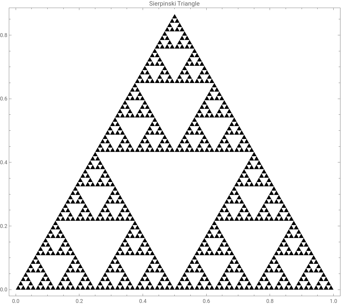
We first begin by defining the coordinates of the triangle on a 2D plane. The ‘generateTriangle’ function allows us to find the midpoint of the edges and then gives back three smaller triangles not including the central area. The ‘Nest’ function calls back the ‘generateTriangle’ six times to perform this action, where each time the triangles get smaller and smaller, which are then flattened into a list and drawn with ‘Graphics’. I will say that I was not able to repeat the function call more than six times because of the The output is a classical Sierpinski triangle.
Triangular and Hexagonal Sierpinski Variants
Triangular and Hexagonal Sierpinski Variants
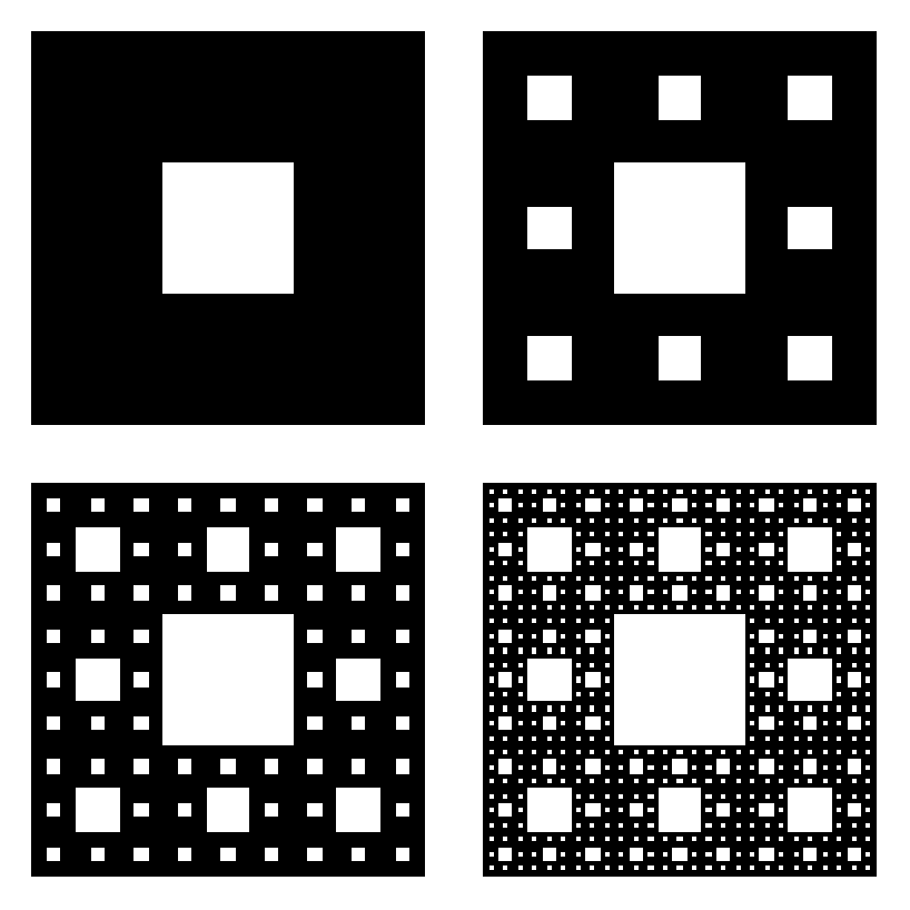
This next part looks at what happens when we replace the triangle with a hexagonal pattern and then apply the subdivision into the six triangular sectors. Repeating this step to create a Sierpinski triangle is very similar to the Sierpinski carpet, which is an image of repeating patterns. Here is an example of a Sierpinski carpet.Shout out to ‘Emerging Technology’ for creating this image and publishing it to the MIT technology review. I will link the proper citation towards the end of this article. Now, back to the Sierpinski variants. This experiment allows me to show how the concept of recursion and repetition can cause special patterns.
triangle=Polygon[{{0,0},{1,0},{0.5,Sqrt[3]/2}}];subdivideTriangle[poly_Polygon]:=Module[{points=First[poly],midpoint12,midpoint23,midpoint31},midpoint12=Mean[{points[[1]],points[[2]]}];midpoint23=Mean[{points[[2]],points[[3]]}];midpoint31=Mean[{points[[3]],points[[1]]}];{Polygon[{points[[1]],midpoint12,midpoint31}],Polygon[{points[[2]],midpoint23,midpoint12}],Polygon[{points[[3]],midpoint31,midpoint23}],Polygon[{midpoint12,midpoint23,midpoint31}]}];recursiveSubdivide[polys_List,n_Integer?NonNegative]:=Nest[Flatten[subdivideTriangle/@#]&,polys,n];result=recursiveSubdivide[{triangle},4];Graphics{EdgeForm[Black],FaceForm[White],result},
Out[]=
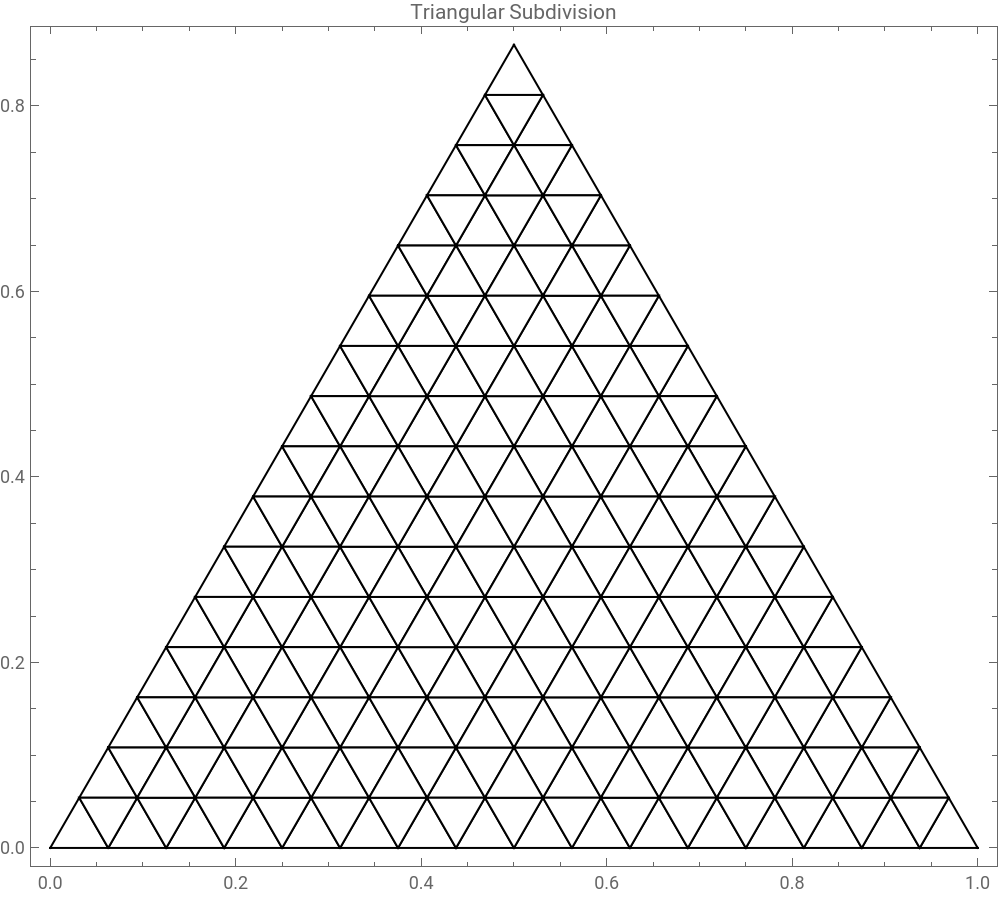
For this part of the project, I first define the equilateral triangle with vertices at (0,0), (1,0), and (0.5, sqrt3/2). The function ‘subdivideTriangle’ takes a polygon and divides it into four smaller triangles by find the midpoint of each side. Specifically, it finds the midpoint between each pair of adjacent vertices and then creates new triangles, three of which are around the original vertex and one is in the center. The ‘recursiveSubdivide’ function uses this method of subdividing and applies it to triangles, nesting the process ‘n’ times to create ever finer subdivisions. If we start with the single starting triangle, the code continues to create recursive subdivisions, which creates a pattern of smaller triangles. Finally, the ‘Graphics’ function will draw this out and print the object you see above.
Let’s look at the same process of subdividing triangles but with another shape, such as a hexagon. The goal of the section below is to look at how hexagonal shapes can be broken down into simple recursive parts to show the similar patterns the it can create. By subdividing hexagons into triangles so that they all share the center of the hexagon, the process can maintain symmetry.
hexagon=Polygon[Table[{Cos[kPi/3],Sin[kPi/3]},{k,0,5}]];subdivideHexagon[poly_Polygon]:=Module[{points=First[poly],center},center=Mean[points];Table[Polygon[{center,points[[k]],points[[Mod[k,Length[points]]+1]]}],{k,Length[points]}]];recursiveSubdivision[polys_List,n_Integer?NonNegative]:=Nest[Flatten[subdivideTriangle/@#]&,polys,n];initialTriangles=subdivideHexagon[hexagon];result=recursiveSubdivision[initialTriangles,3];Graphics{EdgeForm[Black],FaceForm[White],result},
Out[]=
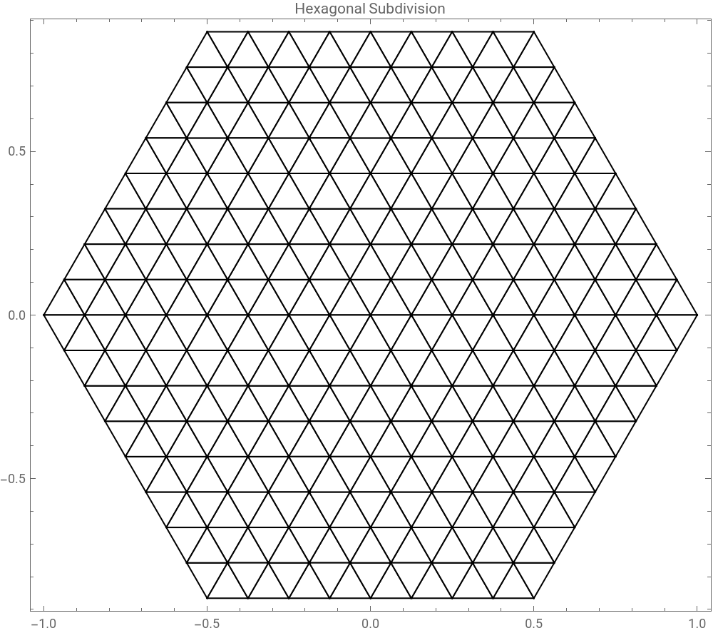
The code starts off by defining a regular hexagon with the center being at (0,0), which is also made by finding the six vertices equally spaced around the center at sixty degree intervals. The function ‘subdivideHexagon’ takes this newly made polygon and finds the centroid by getting the average of the coordinates of the vertices. Then, it subdivides the hexagon into six triangles by connecting the center to each of the adjacent vertices, basically sectioning the hexagon into radial slices. To create a fractal detail in the hexagon, the ‘recursiveSubdivision’ function repeats the midpoint subdivision to the triangles so that each triangle is replaced by four smaller ones. Starting from the six triangles that were created at the starts, the code does three calls of the recursive subdivision. finally, the ‘Graphics’ function displays the results you see above by scaling and framing the hexagon.
Spectral Gaps in a Graph
Spectral Gaps in a Graph
In this part of the project, I will look at spectral graph theory, a theory that studies the relationships in graphs,. Specifically, I will be building a graph where each of the vertex is a triangle corner, and edges connect the adjacent points. The Laplacian spectrum and the eigenvalues of this graph shows the structure and how the shape affects the distribution across the shape. The plot is made by subdivided triangles, which is from the fractal triangle subdivision, and are displayed in ascending order from the vertical axis and indexed along the horizontal axis. In this graph, the black dots show the eigenvalues, the red dots highlight when there are large gaps between the eigenvalues, which are known as spectral gaps, and the blue labels shows the actual eigenvalue at the gap for the location.
starter=Polygon[{{0,0},{1,0},{0.5,Sqrt[3]/2}}];subdivide[poly_Polygon]:=Module[{points=First[poly],midpoint12,midpoint23,midpoint31},midpoint12=Mean[{points[[1]],points[[2]]}];midpoint23=Mean[{points[[2]],points[[3]]}];midpoint31=Mean[{points[[3]],points[[1]]}];{Polygon[{points[[1]],midpoint12,midpoint31}],Polygon[{points[[2]],midpoint23,midpoint12}],Polygon[{points[[3]],midpoint31,midpoint23}],Polygon[{midpoint12,midpoint23,midpoint31}]}];vertices=Union[Flatten[Nest[Flatten[subdivide/@#]&,{starter},3]/.Polygon[pts_]:>pts,1]];edges=Union@Flatten[Table[UndirectedEdge[AssociationThread[vertices->Range[Length[vertices]]][tri[[1,i]]],AssociationThread[vertices->Range[Length[vertices]]][tri[[1,j]]]],{tri,Nest[Flatten[subdivide/@#]&,{starter},3]},{i,3},{j,i+1,3}],2];laplacianMatrix=KirchhoffMatrix[Graph[Range[Length[vertices]],edges,VertexCoordinates->vertices,GraphStyle->"ThickEdge"]];gapIndices=Flatten[Position[Differences[Sort[Eigenvalues[laplacianMatrix]]],x_/;x>0.5]];gapPoints=Transpose[{gapIndices+1,Sort[Eigenvalues[laplacianMatrix]][[gapIndices+1]]}];ListPlotSort[Eigenvalues[laplacianMatrix]],PlotStyle->Black,PlotMarkers->{"●",8},Epilog->{Red,PointSize[0.015],Point[gapPoints],Blue,Table[Text[Style[NumberForm[point[[2]],{4,3}],8,Bold],point,{-1.5,0}],{point,gapPoints}]},
Now you may be wondering, what is this. Well here is the explanation of the code. The code above starts by defining the equilateral triangle using the ‘Polygon’ function to give it points and assign it to the ‘starter’ variable, and then gives a midpoint subdivision process, where each triangle is cut into four smaller pieces by connecting the midpoint o the the edges. This subdivision process happens three times to make a mesh of triangles. Then, undirected edges are made by connected the vertices of in each triangle, which builds a graph showing the mesh of triangles. Furthermore, using the `KirchhoffMatrix` function, we are able to make the Laplacian matrix of the graph to store the eigenvalues. If I did not go over eigenvalues or you may not have known what that is, eigenvalues are vectors that are unchanged even if a transformation occurs. These gaps though, are found by filtering all the different eigenvalues greater than 0.5, which is found ‘gapIndices’. The points are plotted in red and black colors, and the labels are in blue. This graph shows that the structure of the triangle is not random, but actually deliberate.
Apollonian Circle Packing Approximation
Apollonian Circle Packing Approximation
Apollonian packing is a dense arrangement of circles in a space, in such a way where none of the circles overlap. In this section, I created a graph to illustrate such pickings. Instead of triangles, there is a circle that is replaced instead. The center of the circle is the same as the center of the triangle, but is positioned in a way where there are no over flaps. I believe that this project is a very interesting and special way to show how symmetry is present in fractals, more specifically, the Sierpinski shapes.
What you see here is an Apollonian circle packed graph, which was done by drawing circles at the center of what would have been triangles(if we look back at the Sierpinski triangle). First, the program finds the center of where the triangles would have been by doing three sets of subdivisions to a starting triangle. Each center is found by taking the average of the coordinates of the vertices of the triangle. Then, the code finds the minimum distance between any two centers to find what size the circles should to make sure that they do not overlap. The ‘Graphics’ function draws the circles on a graph at the center of the triangle. The radius of each circle has also been adjusted to 45% of the minimum center -to-center length to create a more dense space without overlapping circles.
Section on Fractal Dimension Estimation via Box Counting
Section on Fractal Dimension Estimation via Box Counting
This part of the project uses box-counting methods to find the fractal dimensions, also known as Hausdorff dimensions, of the triangle patterns when they are subdivided. The reason I decided to add this into my project, is not only to explore different parts of subdividing triangles, but to also see what happens at a smaller scales. Specifically, I wanted to learn more about the structure of these subdivided triangles. We see that as time goes on, and the scale gets progressively smaller, we see that the box-counting dimensions slowly start to converge to a point. This convergence gives very strong evidence that this is a fractal, not just visually, but mathematically.
This code first starts of by finding all the vertex points in the polygon through ‘points’. Then, for the smaller sizes of the box, which ranges from 1/2 to 1/256, the algorithm finds how many grid boxes contain at least a single point. Inside the function ‘boxCount’, all points are assigned to specific grid coordinates that will be used in the ‘Floor’ division and removes all duplicates. The output is plotted on a logarithmic graph, where the x-axis shows the box size and the y-axis shoes the box count. The fractal’s dimension is found by finding the negative slope of the best fit line, which is shown below the graph itself. If we take a perfect Sierpinski triangle, the dimension would approach log_2 (3), which is around 1.585, which is something similar that we see here. We were able to find this number as it comes from the Sierpinski triangle recursive construction, where at each step there are three copies of itself scaled by 1/2, giving us the formulas as log(number of copies) / log(scale factor) = log_3 / log_2 = log_2 (3)The result shows us strong evidence, though not proof, that the structure acts like a fractal.
Estimating Fractal Dimension from Spectral Data
Estimating Fractal Dimension from Spectral Data
I began by calculating the number of Laplacian eigenvalues that are less than ‘t’, a threshold. The function ‘numberOfEigenValues[t_]’ does exactly that. The code then generates a table of pairs for all of the ‘t’ values, with each pair looking like this: (Log[t], Log[numberOfEigenValues[t]]). A linear model is then created for this log data, and the slope is calculated using the ‘dimFit’ function, which gives an output of the fractal’s estimated spectral dimensions. This is all displayed on the graph above using ‘ListLinePlot’. The graph specifically depicts the growth of the eigenvalue count, as shown by the staircase-like graph, which provides strong evidence that the behavior is similar to a fractal.
Conclusion
Conclusion
This project investigated the structure of fractals using the recursive subdivision of polygons, particularly triangles. We were able to see the difference between these structures by beginning with a simple Sierpinski triangle and then extending to hexagonal bases. Using Laplacian eigenvalue analysis, we were able to use spectral gaps as evidence of symmetry in the fractals and see how they remained true to pattern at every scale. We also investigated how to estimate fractal dimensions using box-counting. These graphs assisted us in analyzing and obtaining evidence that these fractals are actual fractals. Though it was not concrete proof that those were fractals, it did show us another way to get evidence towards defining these shapes. Overall, the project demonstrated how mathematics can reveal self-similarity and symmetry in certain shapes.
Applications and Extensions
Applications and Extensions
This project has the potential to be extended and applied in many other areas by using the concepts of shape subdivision and spectral analysis. For example, developing a model or graph for a recursive subdivision of triangles as a routing structure, or diving deeper into bandwidth or fault tolerance, can greatly benefit this project in the real world. We also can use eigenvalues and spectral gaps to look at signals traveling from place to place or to investigate how circuit boards work; the possibilities for this project are endless.
Citations
Citations
1.Emerging Technology from the arXivarchive page. ‘Infinity Computer’ Calculates Area Of Sierpinski Carpet Exactly. 19 Mar. 2012.
Keywords
Keywords
-Fractal geometry
-Fractals
-Recursive subdivision
-Sierpinski shapes
-Triangles
-Laplacian graphs
-Spectral gaps
-Fractals
-Recursive subdivision
-Sierpinski shapes
-Triangles
-Laplacian graphs
-Spectral gaps
CITE THIS NOTEBOOK
CITE THIS NOTEBOOK
Investigating fractal triangles and spectral graph analysis in recursive subdivision
by Pavel Pomozov
Wolfram Community, STAFF PICKS, February 20, 2026
https://community.wolfram.com/groups/-/m/t/3642331
by Pavel Pomozov
Wolfram Community, STAFF PICKS, February 20, 2026
https://community.wolfram.com/groups/-/m/t/3642331