Wolfram Cloud Document

Optimization functions

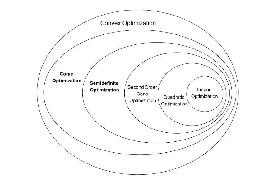
Convex Optimization

A convex optimization problem is one of the form minimize

(x)

subject to

(x)≤0,i=1,2,...,m,

where the functions

(x),...,

(x)





are convex, i.e., satisfy

(αx+βy)≤α

(x)+β

(y)

for all

x,y∈



and all

α,β∈

with

α+β=1,α≥0,β≥0.

Convex Optimization

Minimize

f(x)

, subject to

.x+

=0,

.x+



0,j=1...k

{"NonNegativeCone",n}	n  ≥0	x∈ n  such that x i ≥0
{"NormCone",n}	n 	x∈ n  such that { x 1 ,…, x n-1 }≤ x n
{"SemidefiniteCone",n}	n  +	symmetric positive semidefinite matrices x∈ n×n 
"ExponentialCone"	 exp	x∈ 3  such that x 2 ( x 1 / x 2 )  ≤ x 3 ∧ x 2 ≥0
"DualExponentialCone"	*  exp	x∈ 3  such that - x 1 ( x 2 / x 1 -1)  ≤ x 3 ∧ x 1 <0 or x 1 0∧ x 2 0∧ x 3 0
{"PowerCone",α}	 α	x∈ 3  such that α x 1 1-α x 2 ≥ x 3 ∧ x 1 ≥0∧ x 2 ≥0
{"DualPowerCone",α}	*  α	x∈ 3  such that α ( x 1 /α) 1-α ( x 2 /(1-α)) ≥ x 3 ∧ x 1 ≥0∧ x 2 ≥0

Conic Optimization Models

Beyond Convex: Mixed Integer Conic Optimization

Minimize

c.x

, subject to

.x+

=0,

.x+



0,j=1...k,

∈,j=1,2,…,k,

∈,s=k+1,…,n.

{"NonNegativeCone",n}	n  ≥0	x∈ n  such that x i ≥0
{"NormCone",n}	n 	x∈ n  such that { x 1 ,…, x n-1 }≤ x n
{"SemidefiniteCone",n}	n  +	symmetric positive semidefinite matrices x∈ n×n 
"ExponentialCone"	 exp	x∈ 3  such that x 2 ( x 1 / x 2 )  ≤ x 3 ∧ x 2 ≥0
"DualExponentialCone"	*  exp	x∈ 3  such that - x 1 ( x 2 / x 1 -1)  ≤ x 3 ∧ x 1 <0 or x 1 0∧ x 2 0∧ x 3 0
{"PowerCone",α}	 α	x∈ 3  such that α x 1 1-α x 2 ≥ x 3 ∧ x 1 ≥0∧ x 2 ≥0
{"DualPowerCone",α}	*  α	x∈ 3  such that α ( x 1 /α) 1-α ( x 2 /(1-α)) ≥ x 3 ∧ x 1 ≥0∧ x 2 ≥0

Beyond Convex: Quasi-convex Optimization

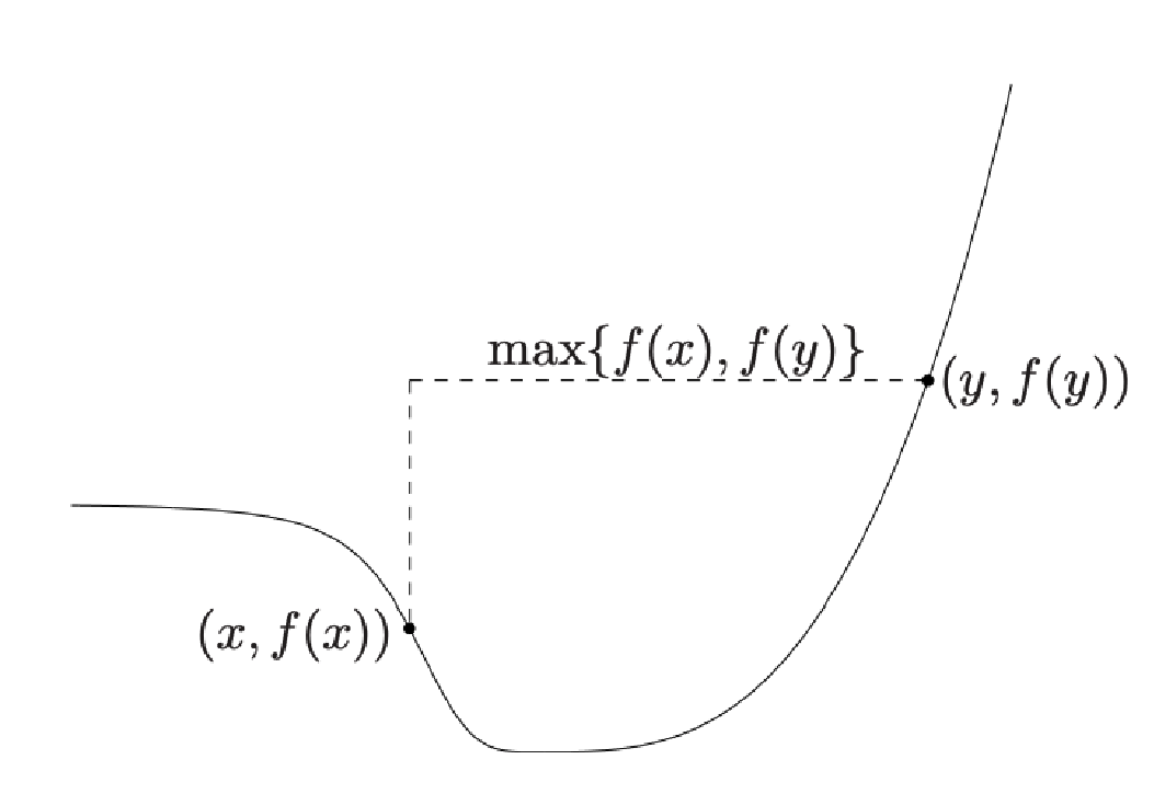
A quasi-convex optimization problem is one of the form minimize

(x)

subject to

(x)≤0,i=1,2,...,m,

where

(x),...,

(x)





are convex, and

(x)

is quasi-convex:

(αx+βy)≤max{

(x),

(y)}

for all

x,y∈



and all

α,β∈

with

α+β=1,α≥0,β≥0.

Beyond Convex: Difference of Convex Optimization

A difference of convex optimization problem is one of the form minimize

(x)-

(x)

subject to

(x)-

(x)≤0,i=1,2,...,m,

where the functions

(x),...,

(x)

and

(x),...,

(x)





are convex

(αx+βy)≤α

(x)+β

(y),

(αx+βy)≤α

(x)+β

(y)

for all

x,y∈



and all

α,β∈

with

α+β=1,α≥0,β≥0.

Methods for Convex Optimization

External Libraries

(*) Except mixed-integer SDP.

Additional methods

◼

LinearOptimization: Simplex, RevisedSimplex, InteriorPoint

◼

QuadraticOptimization: EqualityConstrainedQuadratic, ActiveSetQuadratic and ADMM (for arbitrary precision)

◼

SecondOrderConeOptimization: PolyhedralApproximation, FischerBurmeister (for arbitrary precision)

◼

SemidefiniteOptimization: PolyhedralApproximation, FischerBurmeister (for arbitrary precision)

◼

ConicOptimization: IPOPT(customized for conic)

◼

Mixed-integer Conic: Outer Approximation, ConvexMixedIntegerBranchAndBound

Methods for Constrained Local Optimization

There are a number of methods for unconstrained local optimization (“Gradient”, “ConjugateGradient”, “QuasiNewton”, “Newton”, “LevenbergMarquardt”) but only the following also work with constrained local optimization:

◼

InteriorPoint

◼

IPOPT (machine precision only) - new in version 11

◼

Convex (or give a specific convex or transformable to convex method) - new in version 12

Example with FindMinimum

The constraint function is concave!

So what is the Automatic method here?

Methods for Constrained Global Optimization

◼

Convex (for convex problems)
Can also specify a specific convex (or transformable to convex) method depending on the problem.

◼

Except[“Convex”]
Will not use convex or transformable to convex methods.

Future plans: add general non-convex, non-linear global optimization solvers like Couenne (open-source) and possibly commercial solvers.

Example with NMinimize

A Typical Optimization Example:

The width, height and aspect ratios are constrained to be in a certain range:

A Typical Optimization Example:

Specify the parameters:

Find the dimensions of the individual segments by minimizing the weight:

Visualize the cantilever beam:

A Fitting Example: Basis Pursuit

Use LASSO (L1) regularization to find a sparse fit (basis pursuit):

Here is a signal:

The goal is to approximate the signal with just of few of the thousands of Gabor basis functions:

A Fitting Example: Basis Pursuit

The error is quite small:

Once the important elements of the basis have been found, error can be reduced by finding the least-squares fit to these elements:

An Image Processing Example:

Recover a corrupted image by finding an image that is closest under the total variation norm:

Create a corrupted image by randomly deleting 70% of the data points.

An Image Processing Example:

Find the solution and show the restored image:

Exploring beyond the obvious

We can solve this directly:

Visualize the enclosing ball:

But....What points touch the ball??

Exploring beyond the obvious: Reformulation

Only the extreme points have non-trivial weights:

Exploring beyond the obvious: Use hidden information

Sometimes very useful answers and queries are hidden in plane sight:

Visualize the enclosing ball with the extreme points:

What is a dual and why should I care?

A general minimization problem is:

By using Lagrange multipliers, we can write the optimization problem as:

The Lagrangian dual function (or just the dual problem):

Exploring beyond the obvious: Interpreting the dual

Find the plane that separates two non-intersecting convex polygons:

The hyperplane is constructed as:

Mixed Integer Convex Optimization

The original conic problem is split into two sub-problems:

Outer Approximation Algorithm: An example

Lets solve the following mixed-integer problem:

1. Solve the relaxed conic problem:

2. Find the hyper-plane formed by the dual cone:

Outer Approximation Algorithm: An example

3. Solve the linear sub-problem and get the integer values:

4. Substitute the integer values back into the relaxed conic problem and solve:

5. Find the hyper-plane formed by the dual cone:

6. Repeat step 3-5 adding more hyper-planes:

Tips and Tricks to modelling with integer variables.

Path planning around obstacles:

Find the shortest path between two points while avoiding obstacles. Specify the obstacle:

Extract the half-spaces that form the convex obstacle:

Specify the start and end points of the path:

Path planning around obstacles:

Specify the end point constraints:

Path planning around obstacles:

Find the minimum distance path around the obstacle:

Extract and display the path:

Optimization with Uncertainty: Robust Optimization

Consider a linear optimization problem:

Optimization with Uncertainty: Robust Optimization

Taking uncertainty into account we have:

This is HIGHLY inefficient and sub-optimal!!!

Optimization with Uncertainty.

Find the coefficients associated with each of the basis:

Find fit models for 200 possible realizations of the uncertainty:

Show the envelope of the fit models with the robust fit (black) and the data:

Thank You!

CITE THIS NOTEBOOK

Wolfram R&D LIVE: State of Optimization -- Overview and Tools
by Paritosh Mokhasi
Wolfram Community, STAFF PICKS, May 18 2023
https://community.wolfram.com/groups/-/m/t/2921756