My project at camp consisted in the analysis of companies’ websites by their visual content, understanding the relation of them at site-level, and how various companies are similar in their published images by leveraging this data to build a graph. This is achieved using a combination of web crawling, image analysis via perceptual distance and cluster and signal identification
Web crawling
Web crawling
Our goal with web crawling is to create a graph for each website to then download all the images that we’ll use for the analysis. The data is obtained using the Wolfram Entity Framework to access companies data, which in this case are the corresponding URLs, that are then used to crawl each website up to a certain depth are used to build a graph. The graph is then used to download images that would not be directly accessed, and thus have a bigger picture of the website’s content
In[]:=
companies=,,,,,,,,,;
GetCompanyWebsite takes a company’s entity as input and returns its URL
In[]:=
GetCompanyWebsite[company0_Entity]:=Module[{company=company0,url},(url=company["Website"];Return[If[StringQ[url],url,CanonicalName[url]]])]
For each company, we use the GetCompanyWebsite function to access its URL
In[]:=
urls=Table[GetCompanyWebsite[company],{company,companies}]
Out[]=
{http://www.nestle.com,http://www.glencore.com,http://www.cargill.com,http://www.microsoft.com,http://www.ibm.com,http://www.blyth.com,http://www.cbi.com,https://www.royalgold.com,https://www.tesla.com,https://www.acer.com}
Given a URL, GetWebsiteHyperlinks gives all the hyperlinks in a webpage, excluding the ones which points to other websites
In[]:=
GetWebsiteHyperlinks[url0_String]:=Module[{url=url0},(Return[Select[Import[url,"Hyperlinks"],(StringContainsQ[#,StringTake[StringRiffle[Take[StringSplit[#,"."],{2,-1}],"."],{1,-2}]])&]])]
CrawlWebsite builds a graph of a website’s structure up to a certain depth
In[]:=
CrawlWebsite[url0_String,pagesDepth0_Integer,imageSize0_Symbol:Small]:=Module[{url=url0,pagesDepth=pagesDepth0,imageSize=imageSize0},(Return[NestGraph[GetWebsiteHyperlinks,url,pagesDepth,ImageSize->imageSize]])]
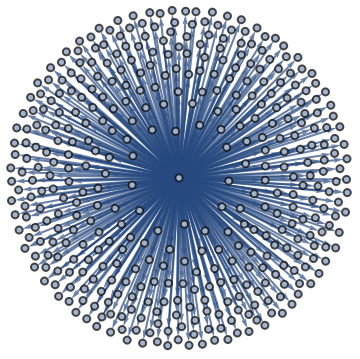
We build a NestGraph to recursively import every link on every given webpage into a graph structure using the CrawlWebsite function. We use pagesDepth to limit the expansion of the graph, since pagesDepth>=3 will result in too much data to handle. pagesDepth=1 will result in a “pivot” pointing to all the direct hyperlinks. We also use maxPages=10 to limit the number of pages on which the images are downloaded for processing speed purposes
In[]:=
pagesDepth=1;
In[]:=
websitesGraphs=Table[url->CrawlWebsite[url,pagesDepth],{url,urls}];Panel[Column[{Panel[Keys[First[websitesGraphs]]],Panel[Values[First[websitesGraphs]]]}]]
Out[]=
We downsize each image to 224, which is the standard size used to train ResNet, in order to save memory. The reason we use a neural network will be explained in later cells
In[]:=
imageSize=224;maxPages=10;
We define the ImportWebsiteImages function, which given a website’s graph, spits out all the images contained in the website
In[]:=
ImportWebsiteImages[websitesGraph0_Graph,imageSize0_Integer:224]:=Module[{websiteGraph=websitesGraph0,imageSize=imageSize0},(Return[Table[ImageResize[image,imageSize],{image,DeleteDuplicates[Select[Join@@Table[Import[url,"Images"],{url,Take[VertexList[websiteGraph],UpTo[maxPages]]}],ImageQ]]}]])]
Then, we apply ImportWebsiteImages to each website we’ve crawled
In[]:=
images=Quiet[Table[Keys[websiteGraph]->ImportWebsiteImages[Values[websiteGraph]],{websiteGraph,websitesGraphs}]];Row[Table[Panel[Column[{Keys[companyImages],Length[Values[companyImages]]}]],{companyImages,images}]]
Out[]=
Images analysis
With image analysis our goal is to port the images to a space where those with similar content will be closer, we do that by analyzing them with a ResNet50 (trough layer 1 to -4). Then perceptual distance is used to determine which images are more similar to others. We finally build a graph of those relations to explore how websites’ image content is structured
We use ResNet as a way to measure distance between images: Two images with similar content but different pixel values will be “judged” by it very similar. This is called perceptual distance
The perceptual distance is defined as =, the average mean squared error between two images’ features
D
i,j
1
W
i,j
H
i,j
W
i,j
∑
x=1
H
i,j
∑
y=1
2
()-()
ϕ
i,j
x
I
x,y
ϕ
i,j
Y
I
x,y
In[]:=
Needs["CUDALink`"];
In[]:=
resnet50:=NetTake[NetModel["ResNet-50 Trained on ImageNet Competition Data"],{1,-4}]visionEncoder=NetAppend[resnet50,{FlattenLayer[]}]
Out[]=
NetChain


In[]:=
batchSize=32;device=If[CUDALink`CUDAQ[],"GPU","CPU"];
The EncodeImages function returns embeddings for a list of images using a given features extractor
In[]:=
EncodeImages[images0_List,featuresExtractor0_,batchSize0_Integer:16,device0_String:If[CUDALink`CUDAQ[],"GPU","CPU"]]:=Module[{images=images0,featuresExtractor=featuresExtractor0,batchSize=batchSize0,device=device0},(Return[Join@@Table[featuresExtractor[imagesBatch,TargetDevice->device],{imagesBatch,Partition[images,UpTo[batchSize]]}]])]
Port images to the latent space using the EncodeImages function. The latent space is a hidden representation of data
In[]:=
imagesEncoded=Table[Keys[companyImages]->Thread[EncodeImages[Values[companyImages],visionEncoder]->Values[companyImages]],{companyImages,images}];Row[Table[Panel[Column[{Keys[imagesEncoded],Length[Values[imagesEncoded]]}]],{imagesEncoded,images}]]
Out[]=
In[]:=
imagesEncoded=Association[imagesEncoded];
In[]:=
imageNeighbors=3;
GetKNearestCompanyImages finds the k nearest images to a given one using perceptual distance, I chose k=3 because I found that separated graphs blend nicely together keeping all the communities’ content intact
In[]:=
GetKNearestCompanyImages[knowledgebase0_Association,company0_String,featuresExtractor0_,image0_Image,k0_Integer]:=Module[{knowledgebase=knowledgebase0,company=company0,featuresExtractor=featuresExtractor0,image=image0,k=k0},(Return[Take[Nearest[Keys[knowledgebase[company]],featuresExtractor[image,TargetDevice->device],k+1],{2,-1}]])]
BuildCompanyImagesGraph builds a graph representing images correlation
In[]:=
BuildCompanyImagesGraph[companyImages0_Rule,imagesEncoded0_Association,featuresExtractor0_,k0_Integer]:=Module[{companyImages=companyImages0,imagesEncoded=imagesEncoded0,featuresExtractor=featuresExtractor0,k=k0},(Graph[Flatten[Table[Table[image->retrievedImage,{retrievedImage,GetKNearestCompanyImages[imagesEncoded,Keys[companyImages],visionEncoder,image,imageNeighbors]}],{image,Values[companyImages]}]],ImageSize->Large])]
We use BuildCompanyImagesGraph to generate the correlation graphs for each company
Associate to each image’s embedding the corresponding company
We then train a dimension reducer to visualize the latent space
We apply the dimension reducer to companiesImages to make a scatter plot of our data
Clusters identification
Clusters identification
Cluster identification is needed to understand relations between companies: Given the concentration of pictures from companies we can understand their relations. Images embeddings are used to identify those clusters in the latent space, that are then used to compute the scores. We then build an interactive graph to see how it changes in relation to the correlation score
We find cluster of similar images and group them
Now we can understand how companies correlates using occurrences in clusters
We group all the correlations to then calculate the final score
Identical but reverse correlations are now removed
We identify the maximum correlation for the manipulate
Create an interactive companies correlation graph based on which images they have on their websites
Signal identification
The goal here is to capture the “signal” that tells us how each of the images are related to the target’s value
The first step is to decide what property we want to work on: We could capture the signal in relation to the revenue, geographical position, or any other measurable property. In this case we want to perform binary classification, so the score will be 1 for the companies that matches our target class (is x a tech company?) and 0 for the others
Now we define a target, which is the value we want to capture the relations in respect to
We model the score in respect to x and y to discover relations to the target
Now we plot the output of targetPredictor in a 3d space
The last step is to test our model on unseen websites
We crawl the unseen websites in the exact same way we did previously
The data is preprocessed to obtain embeddings
We reduce the data to a two-dimensional form
For each image in the unseen websites we run the model to understand what is their score
For each unseen website we learn a distribution
Now we plot the outputs
Conclusion
Conclusion
Through this project we now have a way of comparing websites visual contents both on a intra-site level and inter-site and representing them as graphs. This is useful to construct representation of image data, understand how it relates to other, and highlight a company’s visual communication strategy. We can concluded that even though clustering websites based on the visual content does not yield the best results, it's possible to use that data to extract a "signal" and identify novel websites with similar measurable properties using just an handful of example websites
What may come next
What may come next
The data extracted with this work could be used to understand what sectors a given image style could resemble. It might also be used to discover new visual trends to track how the web is evolving or, in a similar way, how has the internet evolved in the past leveraging archive data
Acknowledgments
Acknowledgments
I would like to thank my mentor, Kurt Gimbel, for his support to the development of this project
Citations
Citations
1
.Perceptual distance (VGG Loss) - Justin Johnson, Alexandre Alahi, Li Fei-Fei, 2016, Stanford University