ORIGINAL ARTICLE: Jerome Goddard, Ratnasingham Shivaji, James T. Cronin, Ecological release and patch geometry can cause nonlinear density–area relationships, Journal of Theoretical Biology (2023), 557, 111325, ISSN 0022-5193, https://doi.org/10.1016/j.jtbi.2022.111325.
A primary driver of species extinctions and declining biodiversity is loss and fragmentation of habitats owing to human activities. Many studies spanning a wide diversity of taxa have described the relationship between population density and habitat patch area, i.e., the density-area relationship (DAR), as positive, neutral, negative or some combination of the three. However, the mechanisms responsible for these relationships remain elusive. In this talk, we will discuss implementation of a reaction-diffusion framework with absorbing boundary conditions to model a habitat specialist dwelling in islands of habitat surrounded by a hostile matrix. We consider patches with both a convex and non-convex geometry. Our results show overall DAR structure can be either 1) positive, 2) positive for small areas and neutral for large, or 3) hump-shaped, i.e., positive for area below a threshold and negative for area above. We will also discuss comparison of our theoretical results with two empirical studies. Close qualitative agreement between theoretical and observed DAR indicates that our model gives a reasonable explanation of the mechanisms underpinning DAR found in those studies.
Setup
Setup
(*Launchkernels*)LaunchKernels[];(*Turnoffwarningregardingnumericalintegration*)Off[NIntegrate::slwcon,NIntegrate::eincr,NIntegrate::ncvbr];ParallelEvaluate[Off[NIntegrate::slwcon,NIntegrate::eincr,NIntegrate::ncvbr];];(*Functiontoreturn(minimumλ-valueforwhichaspeciescansurvive)givenapatchgeometrypatchGEO1*)DetermineE1D=Function[{patchGEO1},NDEigensystem[{-Laplacian[ϕ[x,y],{x,y}],DirichletCondition[ϕ[x,y]0,True]},ϕ[x,y],{x,y}∈patchGEO1,1][[1,1]](*EndoffunctionDetermineE1D*)];(*-------------EndofFunctiontoreturngivenapatchgeometry*)Print["Setup loaded!"];
D
E
1
D
E
1
Setup loaded!
Single Species DAR
Single Species DAR
Convex patch: Disk
Convex patch: Disk
In[]:=
Ω0=Disk[];Region[Ω0]Area[Ω0]
Out[]=

Out[]=
π
Need to resize Ω0 to have unit area.
Need to resize to have unit area.
Ω
0
In[]:=
Ω=RegionResize[Ω0,2/Sqrt[Pi]];Area[Ω]
Out[]=
1
Minimum area requirement for species colonization of a disk:
Minimum area requirement for species colonization of a disk:
Example: E1D for a disk-shaped patch is:
In[]:=
E1D=DetermineE1D[Ω]
Out[]=
18.1686
The minimum area requirement for species colonization of a disk is then E1D/R1, where R1 is the Growth-Diffusion Ratio
In[]:=
R1=1;E1D/R1
Out[]=
18.1686
Define numerical solver for our BVP
Define numerical solver for our BVP
A0 is patch area, R10 is the Growth-Diffusion ratio, and M0 is an initial seed for the BVP solvation method.
In[]:=
soln=ParametricNDSolve[{-Laplacian[u[x,y],{x,y}]A0R10u[x,y](1-u[x,y]),DirichletCondition[u[x,y]0,True]},u,{x,y}∈Ω,{A0,R10,M0},InitialSeeding{u[x,y]M0}]
Out[]=
uParametricFunction


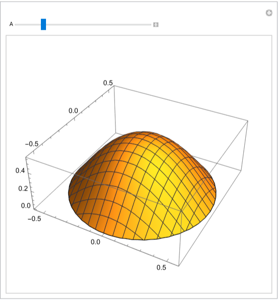
Visually explore solution of BVP: z-axis is population density as a percentage of carrying capacity
Visually explore solution of BVP: z-axis is population density as a percentage of carrying capacity
In[]:=
A=18.18;R1=1;Print["Minimum area requirement is: ",E1D/R1];M=0.6;xypts=RandomPoint[Ω,100];Manipulate[(*Findmaximumu-valueforplotpurposes*)maxu=Max[Table[u[A,R1,M][pt[[1]],pt[[2]]]/.soln,{pt,xypts}]];Plot3D[u[A,R1,M][x,y]/.soln,{x,y}∈Ω,AspectRatioAutomatic,PlotRange->{0,Max[0.01,maxu*1.1]}],{A,E1D*0.9,5*E1D},ContinuousAction->False,SaveDefinitions->True]
Minimum area requirement is: 18.1686
Out[]=
Average density (% of carrying capacity) in Ω is computed using:
Average density (% of carrying capacity) in Ω is computed using:
Given a fixed R1 and M:
In[]:=
ssAD[A_?NumericQ]:=NIntegrate[u[A,R1,M][x,y]/.soln,{x,y}∈Ω]
In[]:=
ssAD[80]
Out[]=
0.533759
Generate DAR:
Generate DAR:
In[]:=
(*Output:DARpointsoftheform:{A,AverageDensityofΩ}*)uDARpts={};(*Setseed&growthrate*)M=0.7;R1=1;(*Pass#1*)Amin1=0.1;ALen1=100;Anum1=50;(*Pass#2*)Amin2=0.1;ALen2=1000;Anum2=50;(*CalculateAmax&Astepforpass#1*)Amax1=Amin1+ALen1;Astep1=(Amax1-Amin1)/Anum1;As1=Range[Amin1,Amax1,Astep1];(*CalculateAmax&Astepforpass#2*)Amax2=Amin2+ALen2;Astep2=(Amax2-Amin2)/Anum2;As2=Range[Amin2,Amax2,Astep2];(*JoinallpassesintooneAsset*)As=Join[As1,As2];(*LoopthroughAsandgenerateDAR*)uDARpts=ParallelMap[If[#<=E1D/R1,{#,0},{#,ssAD[#]}(*Endif#*)]&,As];(*Add{E1D/R1,0}tothelist*)PrependTo[uDARpts,{E1D/R1,0}];(*SortpointsbyA-value*)uDARpts=Sort[uDARpts,#1[[1]]<#2[[1]]&];(*Plotresults*)ListPlot[uDARpts,PlotStyleDirective[Thick,Blue],PlotTheme->"Scientific",JoinedTrue,PlotLegends{"(u, 0)"},FrameLabel->{"A: Patch Area","Average Density (% of Carrying Capacity)"}]
Non-convex patch: Three-bump region (TBR)
Non-convex patch: Three-bump region (TBR)
Minimum area requirement for species colonization of a disk:
Minimum area requirement for species colonization of a disk:
Example: Given E1D for a disk-shaped patch is:
Define numerical solver for our BVP
Define numerical solver for our BVP
A0 is patch area, R10 is the Growth-Diffusion ratio, and M0 is an initial seed for the BVP solvation method.
Visually explore solution of BVP: z-axis is population density as a percentage of carrying capacity
Visually explore solution of BVP: z-axis is population density as a percentage of carrying capacity
Average density (% of carrying capacity) in Ω is computed using:
Average density (% of carrying capacity) in Ω is computed using:
Given a fixed R1 and M:
Generate DAR:
Generate DAR:
Log-Linear Version
Non-convex patch: Actual patch from Sozio et al. 2016
Non-convex patch: Actual patch from Sozio et al. 2016
Import & mesh actual patch from picture in Sozio et al. 2016
Rescale region to have unit area
Minimum area requirement for species colonization of a disk:
Example: Given E1D for a disk-shaped patch is:
Define numerical solver for our BVP
A0 is patch area, R10 is the Growth-Diffusion ratio, and M0 is an initial seed for the BVP solvation method.
Visually explore solution of BVP: z-axis is population density as a percentage of carrying capacity
Visually explore solution of BVP: z-axis is population density as a percentage of carrying capacity
Average density (% of carrying capacity) in Ω is computed using:
Average density (% of carrying capacity) in Ω is computed using:
Given a fixed R1 and M:
Generate DAR:
Generate DAR:
Log-Linear Version
CITE THIS NOTEBOOK
CITE THIS NOTEBOOK
Ecological Release and Patch Geometry
by Jerome Goddard II
Wolfram Community, STAFF PICKS, APRIL 24 2023
https://community.wolfram.com/groups/-/m/t/2906710
by Jerome Goddard II
Wolfram Community, STAFF PICKS, APRIL 24 2023
https://community.wolfram.com/groups/-/m/t/2906710