Briggs-Rauscher MechanismAuthors: Housam Binous and Ahmed Bellagi
Briggs-Rauscher MechanismAuthors: Housam Binous and Ahmed Bellagi
Reactions involved in the BR mechanism:
++⇀2HOI
++⇌2+O
+O+⇌+
+⇀++O
+MA⇀IMA++
where MA is Malonic Acid
Reference:
P. DeKepper and I. R. Epstein, American Chemical Society, Vol. 104, 1982, N. 1, p.49-55
2++⇀HOI+
+
H
-
I
-
IO
3
HIO
2
+
H
-
I
HIO
2
HOI++⇌+O
+
H
-
I
I
2
H
2
-
IO
3
HIO
2
+
H
IO
2
H
2
2⇀HOI++
HIO
2
-
IO
3
+
H
IO
2
H
2
2+
Mn
HIO
2
2+
MnOH
2+
MnOH
H
2
O
2
HO
2
2+
Mn
H
2
2⇀+
HO
2
H
2
O
2
O
2
I
2
+
H
-
I
HOI+⇀+++O
H
2
O
2
O
2
+
H
-
I
H
2
where MA is Malonic Acid
Reference:
P. DeKepper and I. R. Epstein, American Chemical Society, Vol. 104, 1982, N. 1, p.49-55
Symbols in the program:
x1, x2, x3,x4, x5,x6, x7,x8, x9 and x10 in the Mathematica code are the
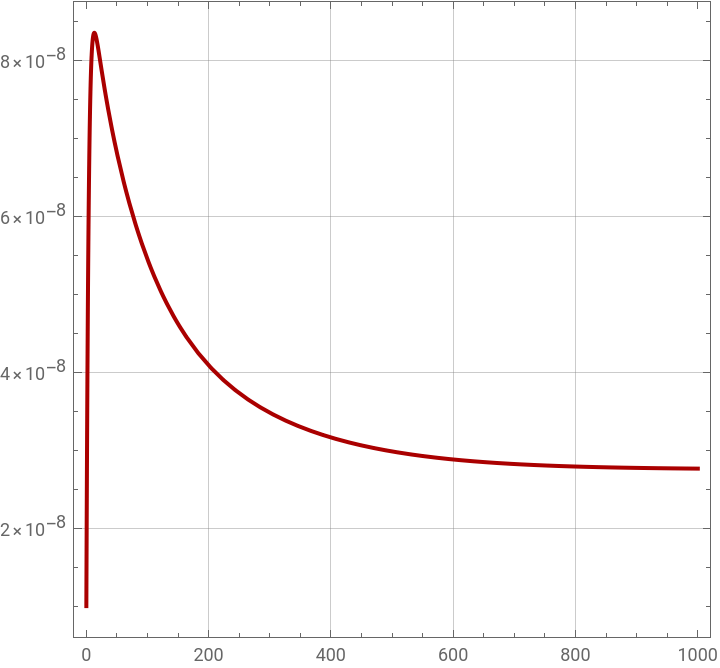
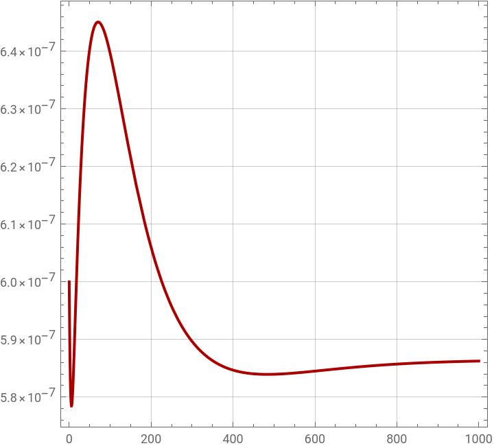
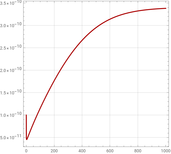
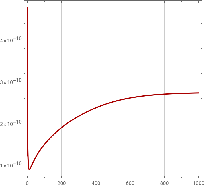
compositions of IO3- , I- , I2 , HIO2 , HOI , IO2 , MnOH2+ , HO2 , MA , H2O2 .
Concentration of H+ is taken as constant equal to h.
The symbols C9, Ki and ki are the different rate constants and constants
appearing in the rate laws (see DeKepper's reference for details).
Xi0 are the 10 concentration of the various components in the feed stream of this open reactor.
The residence time equal to 1/k0=156 s.
A is a constant equal to [Mn2+ ]+[MnOH2+].
Bistability:
The values of X10 and X30 are chosen in order to be in the region of the phase diagram where there is bistability. We get two different steady states when we choose different adequate initial conditions:
Initial condition 1:
x1[0]10^-2, x2[0]10^-8, x3[0]6 10^-7,
x4[0]10^-10, x5[0]10^-10, x6[0]10^-10,
x7[0]10^-13, x8[0]0, x9[0]10^-3, x10[0] 0.
Initial Condition 2:
x1[0]10^-2, x2[0]10^-9, x3[0]6 10^-4,
x4[0]10^-6, x5[0]10^-6, x6[0]10^-7,
x7[0]10^-9, x8[0]0, x9[0]10^-3, x10[0] 0
We give the steady-state values for the different components: Steady state 1 and steady state 2.
Concentration Profiles are given by the links below:
Component : figure 1
Component : figure 2
Component : figure 3
Component : figure 4
Component : figure 5
Component : figure 6
Component : figure 7
The values of X10 and X30 are chosen in order to be in the region of the phase diagram where there is bistability. We get two different steady states when we choose different adequate initial conditions:
Initial condition 1:
x1[0]10^-2, x2[0]10^-8, x3[0]6 10^-7,
x4[0]10^-10, x5[0]10^-10, x6[0]10^-10,
x7[0]10^-13, x8[0]0, x9[0]10^-3, x10[0] 0.
Initial Condition 2:
x1[0]10^-2, x2[0]10^-9, x3[0]6 10^-4,
x4[0]10^-6, x5[0]10^-6, x6[0]10^-7,
x7[0]10^-9, x8[0]0, x9[0]10^-3, x10[0] 0
We give the steady-state values for the different components: Steady state 1 and steady state 2.
Concentration Profiles are given by the links below:
Component
-
I
Component
I
2
Component
HIO
2
Component
HOI
Component
IO
2
Component
+
MnOH
Component
MA
In[]:=
X10=0.04;X20=0;X30=2.510^-6;X40=0;X50=0;X60=0;X70=0;X80=0;X90=0.0015;X100=0.33;h=0.056;A=0.004;k1=1.4310^3;k2=210^10;k3=3.110^12;K3=2.2;k4=7.310^3;K4=1.710^7;k5=610^5;k6=110^4;k7=3.210^4;k8=7.510^5;k9=40;C9=10^4;k0=1/156;k10=37;
Here is solution for the first initial condition
In[]:=
sol=NDSolve[{x1'[t]-k1h^2x2[t]x1[t]-k4hx1[t]x4[t]+K4x6[t]^2+k5x4[t]^2+k0(X10-x1[t]),x2'[t]-k1h^2x2[t]x1[t]-k2hx4[t]x2[t]-k3hx5[t]x2[t]+K3x3[t]+k9x9[t]x3[t]/(1+C9x3[t])+k10x10[t]x5[t]+k0(X20-x2[t]),x3'[t]k3hx5[t]x2[t]-K3x3[t]-k9x9[t]x3[t]/(1+C9x3[t])+k0(X30-x3[t]),x4'[t]k1h^2x2[t]x1[t]-k2hx4[t]x2[t]-k4hx1[t]x4[t]+K4x6[t]^2-2k5x4[t]^2+k6x6[t](A-x7[t])+k0(X40-x4[t]),x5'[t]k1h^2x2[t]x1[t]+2k2hx4[t]x2[t]-k3hx5[t]x2[t]+K3x3[t]+k5x4[t]^2-k10x10[t]x5[t]+k0(X50-x5[t]),x6'[t]2k4hx1[t]x4[t]-2K4x6[t]^2-k6x6[t](A-x7[t])+k0(X60-x6[t]),x7'[t]k6x6[t](A-x7[t])-k7x7[t]x10[t]+k0(X70-x7[t]),x8'[t]k7x7[t]x10[t]-2k8x8[t]^2+k0(X80-x8[t]),x9'[t]-k9x9[t]x3[t]/(1+C9x3[t])+k0(X90-x9[t]),x10'[t]-k7x7[t]x10[t]+k8x8[t]^2-k10x10[t]x5[t]+k0(X100-x10[t]),x1[0]10^-2,x2[0]10^-8,x3[0]610^-7,x4[0]10^-10,x5[0]10^-10,x6[0]10^-10,x7[0]10^-13,x8[0]0,x9[0]10^-3,x10[0]0},{x1,x2,x3,x4,x5,x6,x7,x8,x9,x10},{t,0,2000},AccuracyGoal->15]
Out[]=
x1InterpolatingFunction,x2InterpolatingFunction,x3InterpolatingFunction,x4InterpolatingFunction,x5InterpolatingFunction,x6InterpolatingFunction,x7InterpolatingFunction,x8InterpolatingFunction,x9InterpolatingFunction,x10InterpolatingFunction


In[]:=
Plot[Evaluate[x2[t]/.sol],{t,0,1000},PlotRangeAll,PlotStyle->{Darker@Red,Thick},Frame->True,AspectRatio->1,GridLines->Automatic]
Out[]=
In[]:=
Plot[Evaluate[x3[t]/.sol],{t,0,1000},PlotRangeAll,PlotStyle->{Darker@Red,Thick},Frame->True,AspectRatio->1,GridLines->Automatic,PlotStyle->{Darker@Red,Thick},Frame->True,AspectRatio->1,GridLines->Automatic]
Out[]=
In[]:=
Plot[Evaluate[x4[t]/.sol],{t,0,1000},PlotRangeAll,PlotStyle->{Darker@Red,Thick},Frame->True,AspectRatio->1,GridLines->Automatic,PlotStyle->{Darker@Red,Thick},Frame->True,AspectRatio->1,GridLines->Automatic]
Out[]=
In[]:=
Plot[Evaluate[x5[t]/.sol],{t,0,1000},PlotRangeAll,PlotStyle->{Darker@Red,Thick},Frame->True,AspectRatio->1,GridLines->Automatic,PlotStyle->{Darker@Red,Thick},Frame->True,AspectRatio->1,GridLines->Automatic]
Out[]=
In[]:=
Plot[Evaluate[x6[t]/.sol],{t,0,1000},PlotRangeAll,PlotStyle->{Darker@Red,Thick},Frame->True,AspectRatio->1,GridLines->Automatic,PlotStyle->{Darker@Red,Thick},Frame->True,AspectRatio->1,GridLines->Automatic]
Out[]=
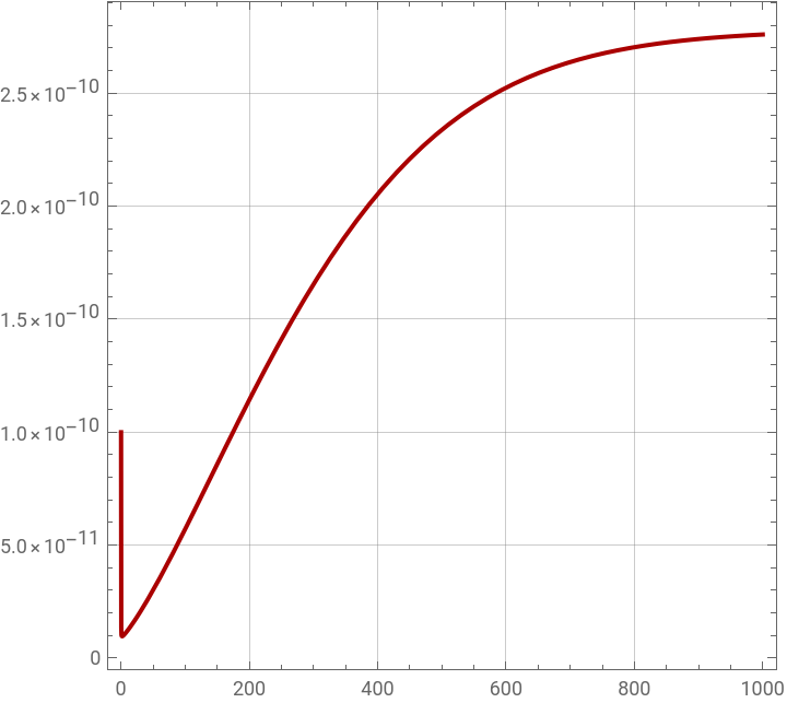
Steady State Values for the first initial condition
Here is the solution for the second initial condition
Steady State Values for the second initial condition
Comparison of the concentration profiles for the first and second initial condition.