Overview
Overview
This notebook presents some unusual ways to look at high frequency stock market price data, including, a simple intraday volatility measure, which I posted recently. The database was collected over more than a year consisting of minute data for the SPY ETF, with price and volume elements for each minute: {dateTime, open, high, low, close, volume}. Only the regular trading hours are included in a list for each day. The SPY ETF was chosen because it is very actively traded and represents most of the capital in the U.S. stock market so that it can be used to assess market trends and volatility. The data is embedded in the notebook so that it may be used in other ways. Unfortunately the collection is not very long. It would be a nice project for the Wolfram Data Repository to make data like this available for a long history, say since 2000, which would include three market crashes for analysis.
Data for this notebook
Data for this notebook
The data are embedded in the notebook as a zipped file converted to a ByteArray. Feel free to explore it in more detail. ByteArrayToString[] doesn’t seem to work here. The following two lines of code extract it.
In[]:=
byteString=FromCharacterCodeNormalByteArray;minData0=ImportString[byteString,{"ZIP","spyMinute.m"}];
Each list in the data is a regular trading day with each minute of data in the format :{dateTime, open, high, low, close, volume}.
In[]:=
minData0[[1]][[1]]minData0[[-1]][[-1]]
Out[]=
,389.89,389.95,389.59,389.76,1352931
Out[]=
,389.65,389.93,389.41,389.6,2949720
The data set contains one short trading day which is removed so all the days will be alike. There are 292 trading days in the remaining data set.
In[]:=
minData=Select[minData0,Length[#]==390&];Length[minData]
Out[]=
292
This convoluted step converts each price {open, high, low, close} to a separate price with a date timestamp which will be handled by the FractalDC algorithm.
In[]:=
minData1=Flatten[{{#1,#2},{#1,#4},{#1,#3},{#1,#5}}&@@@#,1]&/@minData;
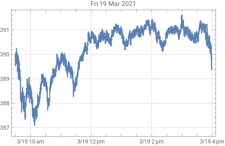
Plot of all the prices in the first day.
In[]:=
plot1=DateListPlot[minData1[[1]],GridLinesAutomatic,PlotRange->All,PlotLabel->DateString[minData1[[1]][[1]][[1]],"DateShort"]]
Out[]=
FractalDC algorithm
FractalDC algorithm
The FractalDC (DC is for data compression) algorithm is used recursively. It looks at the data set, four points at a time and decides whether a point represents a peak or a valley in the four point set and discards the points which are not a peak or a valley. In this way all the local maxima and minima are preserved. The algorithm also preserves the first and last points. In this way if the algorithm were run recursively until there was no further discarding of points, it would be left with the {first, max, min, last} data points. The max and min will be in the order they occurred. The code is below. If each row of data processed by algorithm is a vector, the program operates on the numerical value of the last column of the data. The algorithm does not change of the data it only picks the local extrema out of the sample.
FractalDC Code
In[]:=
Clear[FractalDC];FractalDC[data_]:=Module{d,i=1,positions,len,d0,d1,d2,d3},(*thisstructurewithStuffBag[]isfasterthanAppendTo[]*)positions=Internal`Bag[];len=Length[data];(*thelastcolumnofdataisassumedtocontaintheinformationwiththetrend*)d=If[Length[Dimensions[data]]>1,data[[All,-1]],data];Whilei≤len-3,{d0,d1,d2,d3}=Take[d,{i,i+3}];Internal`StuffBag[positions,i];i=
;;(*addlatestpoint*)Internal`StuffBag[positions,i];(*checkd2*)If[ilen-2&&(d2>d0&&d2>d1&&d2≥d3)||(d2<d0&&d2<d1&&d2≤d3),Internal`StuffBag[positions,i+1]];(*don'tloselastdatapoint*)If[Internal`BagPart[positions,-1]<len,Internal`StuffBag[positions,len]];data[[Internal`BagPart[positions,All]]];
|
In[]:=
fractal6=Nest[FractalDC,#,6]&/@minData1;
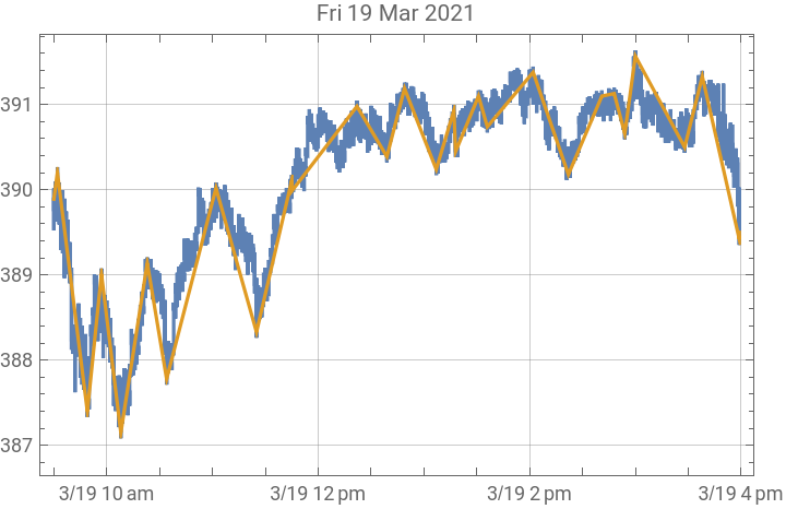
After running the algorithm 6 times recursively on all the days in the data set, this is what is left of the first day’s data in orange. The idea is to try to pick out what a computerized trading algorithm might see as profit opportunities. The algorithm isn’t perfect to the eye, but it does provide a new method of sampling that does include all the local minima and maxima. Explore the data by looking at more days.
In[]:=
plot2=DateListPlot[fractal6[[1]],PlotStyle->ColorData[97][2]];Show[plot1,plot2]
Out[]=
Fractal log returns
Fractal log returns
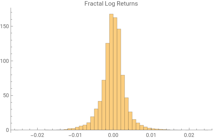
The following step converts the selected intraday prices into log returns. The between day changes are not included because I am interested only in the intraday and how the intraday trading leads to price formation. Then combining all the intraday log returns, there is a large data set to analyze
In[]:=
lr6=Flatten[Differences[Log[#[[All,2]]]]&/@fractal6];Length[lr6]
Out[]=
8325
455520 prices have been sampled to a subset of 8617, from which 8325 intraday log returns were obtained.
In[]:=
Total[Length/@minData1]Total[Length/@fractal6]
Out[]=
455520
Out[]=
8617
In[]:=
plot2=Histogram[lr6,Automatic,"PDF",PlotRange->All,PlotLabel->"Fractal Log Returns"]
Out[]=
Power tail analysis
Power tail analysis
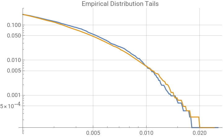
A log log plot of the CDF and reversed CDF tails becomes fairly linear to the eye at about the p 0.005 level for each tail and they appear to be symmetric.
In[]:=
ed=EmpiricalDistribution[lr6];LogLogPlot[{CDF[ed,-x],1-CDF[ed,x]},{x,0.002,Max[Abs[lr6]]},PerformanceGoal"Speed",GridLinesAutomatic,PlotRangeAll,PlotLabel"Empirical Distribution Tails"]
Out[]=
For tail fitting I will use the largest absolute values of a little less than 1% of the data.
In[]:=
Length[lr6]0.01%
Out[]=
8325
Out[]=
83.25
Power tails can be analyzed using a transformation from a Pareto to an exponential distribution. Using the Log[tail] data a quantile plot can be used to see if the relationship is linear. The slope of the line is the power tail exponent α, and a trick can use the plot to calculate the slope from the plot if Method{“ReferenceLineMethod””Fit”} is used.
Estimate α from QuantilePlot.
A better estimate for α can probably be obtained by fitting log[tail] to an exponential distribution by maximum likelihood.
Estimate α by evaluating the empirical characteristic function of the log tail to an interesting version of the exponential distribution characteristic function at a single point. This formula is derived here: Hacking a complex function with Mathematica. The tail information is apparently very close to t = 0 for the characteristic function, but the equation is degenerate at t = 0, where the characteristic function is always equal to 1.
What is the actual distribution to model fractal returns?
What is the actual distribution to model fractal returns?
There probably isn’t one. The fractal sampling exaggerates the serial dependence of the magnitude of the data. The process is not random. The FractalDC algorithm is essentially a signal processing algorithm which transforms the daily market signal and its distribution properties. This particular algorithm effectively removes return data from the middle of the distribution and preserves the extreme prices.
This looks at the returns at the close of each minute of the day without any processing.
The power tail of the log returns at the close of each minute are about the same because the FractalDC algorithm preserves the order of the prices and the extrema.
Minute volume
Minute volume
One of the reasons for using the fractal processing on these data is that the minute sampling is problematic, because much larger numbers of shares are traded at the opening and closing of the trading day. Since the minute data contain the high and low of each minute, the extreme price points are preserved and these can be picked as data points. The blip in volume at minute 270 is due to the Federal Reserve Open Market Committee’s practice of releasing information on Wednesdays at 14:00 eastern time.
FOMC meeting day
FOMC meeting day
Here is a look at trading on the last FOMC meeting day. On meeting days volatility typically explodes when the decision is released.
The next day average volatility remained higher than the previous morning and the market reversed direction.