In this project, we attempt to characterize mobile automata in the form of network graphs. By applying dimension reduction techniques, we transform these high-dimensional network graphs into a simplified 2D space. Our findings reveal distinct clusters of rules, each exhibiting unique behaviors, thus opening avenues for further exploration and classification within the fascinating domain of mobile automata.
Introduction
Introduction
Cellular automata are models composed of “colored” cells (e.g., black and white), on a grid that evolve over time according to specific rules based on the states of neighboring cells. These automata, which are central to Stephen Wolfram’s book “A New Kind of Science” (NKS) demonstrate that even simple rules can generate complex patterns, providing a potential framework for understanding the intricate workings of the universe. In contrast to the parallel updating mechanism in cellular automata, mobile automata introduce a variation where only a single “active” cell evolves at each step. In mobile automata, this active cell not only updates its state, but also its position based on the rules. Cellular automata have been extensively researched and characterized. Indeed, during the 1980s, Stephen Wolfram provided a significant contribution by proposing a classification system for cellular automata behavior. He categorized them into four distinct classes based on the outcomes observed when the system evolved from a disordered initial state. On the other hand, mobile automata remain a less-explored territory. Thus, our work seeks to uncover new insights about the behavior and characteristics of mobile automata.
Preliminaries
Preliminaries
Defining the rule
Defining the rule
A mobile automaton, much like its cellular counterpart, consists of a line of cells, each of which can be in one of two possible states, represented by two colors. However, a defining characteristic of mobile automata is the presence of a single “active cell” at any given step, indicated by a black dot. The rule governing a mobile automaton applies exclusively to this active cell. It considers the state of the active cell and its immediate neighbors, and based on this, the rule specifies two things: the new state of the active cell and the direction of the active cell’s movement, either to the left or the right. This rule forms the basis of the unique evolution and behavior seen in mobile automata, continuously influencing the state and movement of the active cell throughout the system’s operation. Throughout the discussion in this notebook, we assume there are only two colors (black and white).
One natural question is to ask how many rules there are. Each cell – the active one and its neighbors – can be in one of two states (black or white), generating eight possible combinations (2^3 = 8). For each combination, or scenario, the next step requires the specification of two aspects: the active cell’s new color and its movement direction. This leads to 2 (for color) x 2 (for direction) = 4 possibilities per scenario. Considering these possibilities across all eight scenarios, we obtain 4^8 = 65536 potential rules. Alternatively, we could view it as 2^8 (for color) x 2^8 (for direction) = 65536 possible rules. This perspective forms the basis that a rule can be written in the form of {i, j}, where i and j each ranges from 0 to 255, with i specifying the direction and j specifying the color.
The figure below demonstrates this concept with 1 particular rule out, {35, 57}.
Rule icons for a mobile automaton rule {35, 57}.
In[]:=
ResourceFunction["MobileAutomatonRulePlot"][{35,57}]
Out[]=

Specifying initial condition and time
Specifying initial condition and time
Having specified a rule, our next step involves setting the initial condition (i.e., the colors of the cells at time 0) and determining the duration (time) for which we wish to run the mobile automaton. For instance, we could set the rule as {35, 57}, initialize all cells to white (represented by 0’s), and allow the system to evolve for 60 steps.
Here’s how we could represent this:
Here’s how we could represent this:
In[]:=
rule={35,57};init={ConstantArray[0,41],20};t=60;
We can visualize the evolution of this mobile automaton using the ResourceFunction from the Wolfram Function Repository and the ArrayPlot function:
In[]:=
ArrayPlot[ResourceFunction["MobileAutomaton"][rule,init,t][[All,1]]]
Out[]=
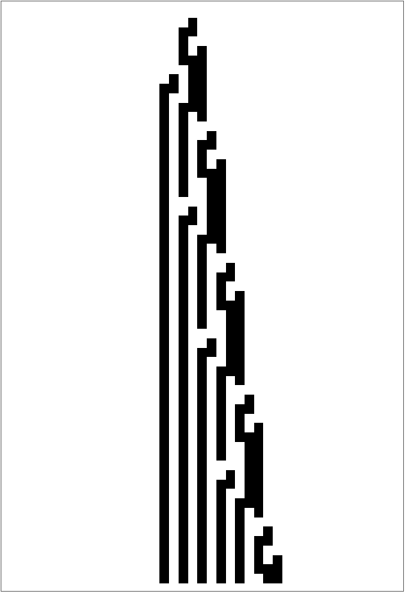
After specifying the rule, initial condition, and the time, we can run the mobile automaton and store the result in a variable, say, obj:
In[]:=
obj=ResourceFunction["MobileAutomaton"][rule,init,t];
This object now contains the entire evolution of our mobile automaton over the specified time.
We can also transform this evolution into a network structure using the MAToNet function implemented in the NKS book and store it in a variable called net. The MAToNet function essentially creates a graph where nodes represent cell configurations and edges represent transitions between configurations:
We can also transform this evolution into a network structure using the MAToNet function implemented in the NKS book and store it in a variable called net. The MAToNet function essentially creates a graph where nodes represent cell configurations and edges represent transitions between configurations:
In[]:=
net=MAToNet[obj[[All,2]]];
Next, we extract unique connections between nodes in the network using the DeleteDuplicates function. This operation is performed on the flattened array of key-value pairs generated by the KeyValueMap function:
In[]:=
cn=DeleteDuplicates[Flatten[KeyValueMap[Thread[#1->#2]&,Association[net]]]];
Finally, we can visualize this network using the Graph function. We use the GraphLayout -> “LayeredDigraphEmbedding” option to arrange the graph’s nodes in a layered manner:
In[]:=
plot=Graph[cn,GraphLayout->"LayeredDigraphEmbedding"]
Out[]=
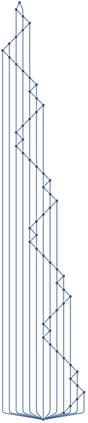
Given the example above, we’ve visualized a single network graph resulting from rule {37, 57} after 60 steps. But let’s recall that we have an enormous array of potential rules—approximately 65,000 in total. Manually inspecting every possible network graph would be an inordinately time-consuming task. Are there more efficient ways we could categorize and compare these graphs? Can we distill the complex structures of these network graphs into a simpler form that still captures their key characteristics? This motivates the next subsection on dimension reduction.
Dimensional reduction
Dimensional reduction
Dimension reduction is a powerful technique, often utilized to project high-dimensional data (e.g., images) into a lower-dimensional space. Methods like Principal Component Analysis (PCA) are commonly employed for this purpose. When dealing with high-dimensional features, such as the network graphs of our mobile automata, dimension reduction allows us to visualize the proximity between these complex structures in a simpler 2D space. This can simply be done using the FeatureSpacePlot function. As a simple example, we can use FeatureSpacePlot to visualize letters on the 2D space. First we could use
In[]:=
imgs=Rasterize/@Alphabet[]
Out[]=
,

,

,

,

,

,

,

,

,

,

,

,

,

,

,

,

,

,

,

,

,

,

,

,

,


which turns the Alphabets into images. Then we could simply do
In[]:=
FeatureSpacePlot[imgs]
Out[]=
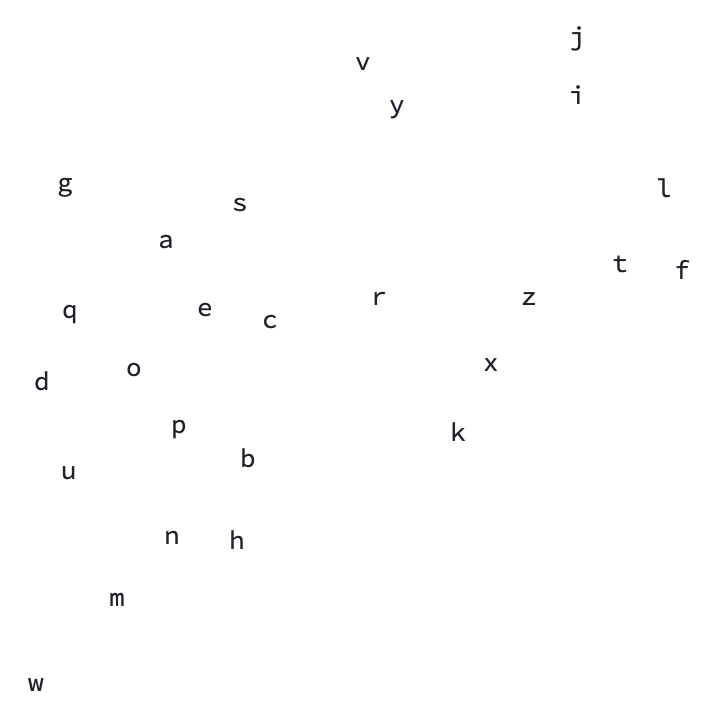
and we see it actually puts alphabets that are more alike into a more proximal 2D space.
Dimension reduction for understanding graphs
Dimension reduction for understanding graphs
In the previous section, we showed briefly how dimension reduction techniques can be used in analyzing complex, high-dimensional data. The fundamental appeal of these methods lies in their ability to simplify data interpretation and comparison. In the context of our study, dimension reduction can be a powerful tool for exploring and understanding the network graphs corresponding to the extensive array of mobile automaton rules.
We can generate the full set of 65536 rules with the following code:
We can generate the full set of 65536 rules with the following code:
In[]:=
rules=Flatten[Table[{i,j},{i,0,255},{j,0,255}],1];
However, due to computational constraints, visualizing all these rules on a 2D plot can be quite challenging. To circumvent this, we can randomly sample a subset of these rules (for instance, a 1000 of them) without replacement. This approach provides us with a manageable and yet representative sample to work with. We set a seed for reproducibility of results:
SeedRandom[20230707];sub=RandomSample[rules,1000];
Next, we specify the initial condition and the time, applying these variables to all the 1000 chosen rules using the Table function:
In[]:=
init={ConstantArray[0,103],52};t=50;objs=Table[ResourceFunction["MobileAutomaton"][rule,init,t],{rule,sub}];nets=Table[MAToNet[obj[[All,2]]],{obj,objs}];cns=Table[DeleteDuplicates[Flatten[KeyValueMap[Thread[#1->#2]&,Association[net]]]],{net,nets}];plots=Table[Graph[cn,GraphLayout->"LayeredDigraphEmbedding"],{cn,cns}];imgs=Rasterize/@plots;FeatureSpacePlot[Table[imgs[[i]]->sub[[i]],{i,Length[imgs]}],LabelingFunction->(Placed[Dynamic[#],Tooltip]&),ImageSize->Large]

The visualization indeed reveals clear clustering among the rules. At first glance, we can discern at least 13 distinct clusters. This suggests that different rules yield networks with unique characteristics, and these shared traits are what group them together into clusters in our 2D space!
Moreover, by enlarging the figure and adding labels to the plots, we can take a closer look at the specific rules that constitute each cluster.
Moreover, by enlarging the figure and adding labels to the plots, we can take a closer look at the specific rules that constitute each cluster.
Concluding remarks
Concluding remarks
In this project, we’ve uncovered multiple clusters of rules within mobile automata, each demonstrating distinct behaviors. These findings shed light on the potential diversity and complexity inherent in such systems. However, our exploration is just the beginning. Further investigations are necessary to classify and fully comprehend the various behaviors exhibited by these rules, which could pave the way for fascinating discoveries in the realm of mobile automata.
Keywords
Keywords
◼
Mobile automata
◼
Causal network
◼
Dimension reduction
Acknowledgment
Acknowledgment
I would like to express my gratitude to my mentor, Eric James Parfitt, for his extensive knowledge of the Wolfram Language and his invaluable support throughout this project. Special thanks to Stephen Wolfram for assigning this captivating project to me and for providing me with this exceptional opportunity. The experience has been eye-opening!
CITE THIS NOTEBOOK
CITE THIS NOTEBOOK
Exploration and Characterization of Mobile Automata
by Lap Sum Chan
Wolfram Community, STAFF PICKS, 13 July, 2023
https://community.wolfram.com/groups/-/m/t/2960211
by Lap Sum Chan
Wolfram Community, STAFF PICKS, 13 July, 2023
https://community.wolfram.com/groups/-/m/t/2960211