Separation of CO2 from a mixture containing CH4, C2H6 and C3H8
Authors: Housam Binous and Ahmed Bellagi
Separation of CO2 from a mixture containing CH4, C2H6 and C3H8
Authors: Housam Binous and Ahmed Bellagi
Authors: Housam Binous and Ahmed Bellagi
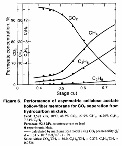
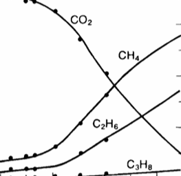
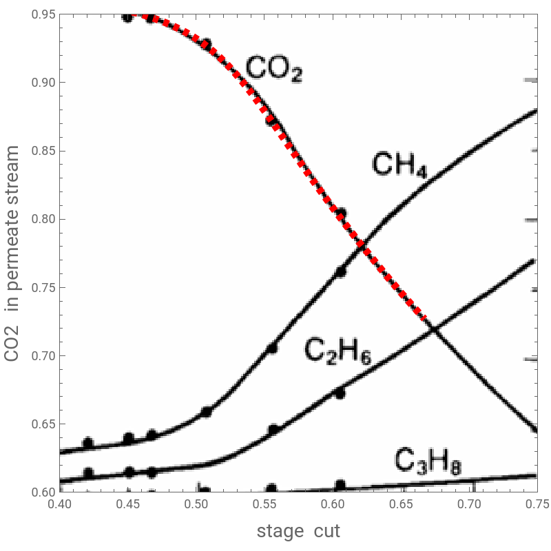
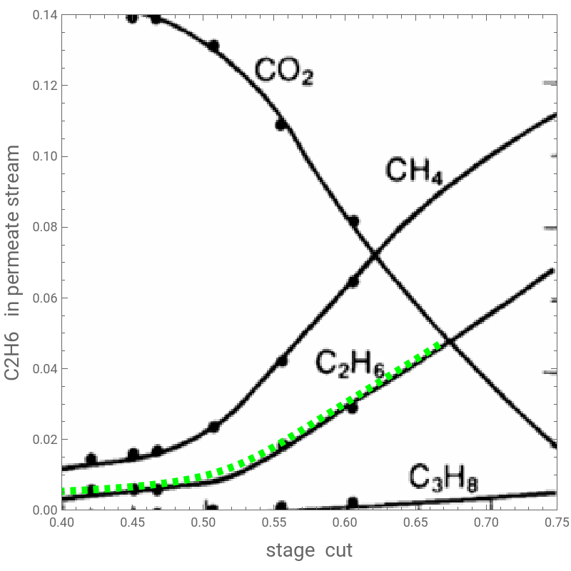
In Ref. 1, Pan studied the separation of CO2 from a mixture of CH4, C2H6 and C3H8 using asymmetric cellulose acetate hollow-fiber membrane. Here, we successfully reproduce Fig. 6 of Ref. 1 using a counter-current gas permeation module and the methodology described in detail in Ref. 2.In this latter figure, Pan depicted the mole fractions of CO2, CH4, C2H6 and C3H8 in the permeate stream versus the stage cut. We also provide the membrane area versus stage cut.References:[1] Pan, C.Y. (1986), Gas separation by high-flux, asymmetric hollow-fiber membrane. AIChE J., 32: 2020-2027. https://doi.org/10.1002/aic.690321212[2] H . Binous, U . Zahid and A . Bellagi, Modeling for Multi - component Gas Permeation with Orthogonal Collocation and Arc - Length Continuation, Chemistry Africa (2024) . https://doi .org/10.1007/s42250-024-01167-y
In[]:=
Out[]=
{xA[1]0.0890573,xB[1]0.480475,xC[1]0.295095,xA[2]0.090303,xB[2]0.479919,xC[2]0.294634,xA[3]0.0941187,xB[3]0.478206,xC[3]0.293227,xA[4]0.100736,xB[4]0.475198,xC[4]0.290808,xA[5]0.110522,xB[5]0.470673,xC[5]0.287273,xA[6]0.123943,xB[6]0.464352,xC[6]0.282493,xA[7]0.141479,xB[7]0.455934,xC[7]0.276336,xA[8]0.163496,xB[8]0.445175,xC[8]0.268714,xA[9]0.190074,xB[9]0.431978,xC[9]0.259632,xA[10]0.220837,xB[10]0.416494,xC[10]0.249241,xA[11]0.254861,xB[11]0.399172,xC[11]0.23786,xA[12]0.290738,xB[12]0.380735,xC[12]0.225957,xA[13]0.326786,xB[13]0.362071,xC[13]0.214077,xA[14]0.361335,xB[14]0.344074,xC[14]0.202754,xA[15]0.392966,xB[15]0.32752,xC[15]0.192432,xA[16]0.420635,xB[16]0.312984,xC[16]0.183434,xA[17]0.443678,xB[17]0.300843,xC[17]0.17596,xA[18]0.461739,xB[18]0.291307,xC[18]0.170114,xA[19]0.474665,xB[19]0.284471,xC[19]0.165937,xA[20]0.482418,xB[20]0.280368,xC[20]0.163433,yA[2]0.813375,yB[2]0.157469,yC[2]0.0267587,yA[3]0.817619,yB[3]0.153904,yC[3]0.0261355,yA[4]0.824463,yB[4]0.148155,yC[4]0.025132,yA[5]0.833561,yB[5]0.140509,yC[5]0.0238,yA[6]0.844445,yB[6]0.131358,yC[6]0.0222102,yA[7]0.856543,yB[7]0.121182,yC[7]0.0204476,yA[8]0.869226,yB[8]0.110507,yC[8]0.0186048,yA[9]0.881872,yB[9]0.0998582,yC[9]0.0167726,yA[10]0.893932,yB[10]0.0896968,yC[10]0.0150303,yA[11]0.904988,yB[11]0.0803769,yC[11]0.0134375,yA[12]0.914777,yB[12]0.072121,yC[12]0.0120308,yA[13]0.923187,yB[13]0.0650245,yC[13]0.0108251,yA[14]0.930226,yB[14]0.0590825,yC[14]0.00981811,yA[15]0.935979,yB[15]0.0542246,yC[15]0.00899661,yA[16]0.940567,yB[16]0.0503488,yC[16]0.0083424,yA[17]0.94412,yB[17]0.0473468,yC[17]0.00783645,yA[18]0.946756,yB[18]0.0451198,yC[18]0.00746157,yA[19]0.948569,yB[19]0.0435876,yC[19]0.00720387,yA[20]0.949629,yB[20]0.0426916,yC[20]0.00705327,yA[21]0.949977,yB[21]0.0423969,yC[21]0.00700374,q[2]0.541024,q[3]0.543872,q[4]0.548809,q[5]0.556128,q[6]0.566244,q[7]0.579688,q[8]0.597061,q[9]0.618959,q[10]0.645834,q[11]0.677835,q[12]0.714644,q[13]0.755378,q[14]0.798589,q[15]0.842368,q[16]0.884528,q[17]0.922812,q[18]0.955096,q[19]0.97956,q[20]0.994816,theta0.459906,0.811938,0.158676,0.0269699,0.00241614}
y
PAi
y
PBi
y
PCi
y
PDi
In[]:=
In[]:=
SYS=Join[sys/.functions,{aux},init,initdev];SOL=Quiet@NDSolve[SYS,unknown1,{s,-10,10},AccuracyGoal5];
In[]:=
pA=ParametricPlot[{theta[s],yA[Np+1][s]}/.SOL[[1]],{s,-10,4.95},PlotRange{{0.4,0.75},{0.6,0.95}},FrameTrue,GridLinesAutomatic,AspectRatio1,PlotStyle{Thickness[0.015],Dashed,Red},FrameTrue,FrameLabel{Style["stage cut",14],Style["CO2 in permeate stream",14]}];pB=ParametricPlot[{theta[s],yB[Np+1][s]}/.SOL[[1]],{s,-10,4.95},PlotRange{{0.4,0.75},{0,0.35}},FrameTrue,GridLinesAutomatic,AspectRatio1,PlotStyle{Thickness[0.015],Dashed,Blue},FrameTrue,FrameLabel{Style["stage cut",14],Style["CH4 in permeate stream",14]}];pC=ParametricPlot[{theta[s],yC[Np+1][s]}/.SOL[[1]],{s,-10,4.95},PlotRange{{0.4,0.75},{0,0.14}},FrameTrue,GridLinesAutomatic,AspectRatio1,PlotStyle{Thickness[0.015],Dashed,Green},FrameTrue,FrameLabel{Style["stage cut",14],Style["C2H6 in permeate stream",14]}];pD=ParametricPlot[{theta[s],1-yA[Np+1][s]-yB[Np+1][s]-yC[Np+1][s]}/.SOL[[1]],{s,-10,4.95},PlotRange{{0.4,0.75},{0,0.14}},FrameTrue,GridLinesAutomatic,AspectRatio1,PlotStyle{Thickness[0.015],Dashed,Magenta},FrameTrue,FrameLabel{Style["stage cut",14],Style["C3H8 in permeate stream",14]}];
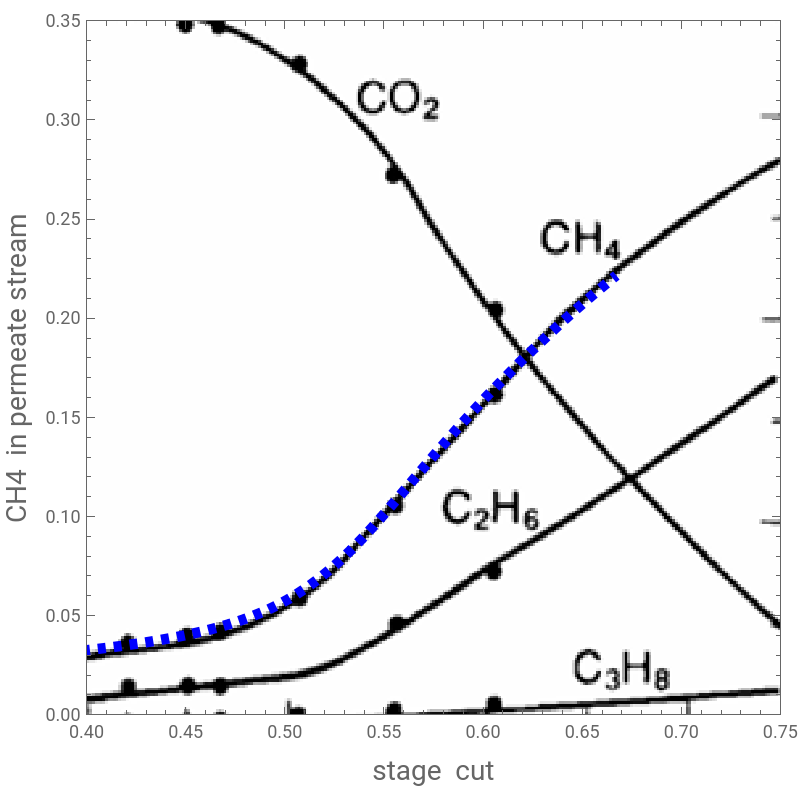
Comparison between our results (colored dashed curves) and Figure 6 of Ref. 1 indicates close agreement, which provides a validation of the methodology described in Ref. 2.
Comparison between our results (colored dashed curves) and Figure 6 of Ref. 1 indicates close agreement, which provides a validation of the methodology described in Ref. 2.
In[]:=
img=
;
In[]:=
Show[pA,ImageSize400{1,1},Prolog{Raster[ImageData[img,DataReversedTrue],{Scaled[{0.00,0.00}],Scaled[{1,1}]}]}]
Out[]=
In[]:=
Show[pB,ImageSize400{1,1},Prolog{Raster[ImageData[img,DataReversedTrue],{Scaled[{0.00,0.00}],Scaled[{1,1}]}]}]
Out[]=
In[]:=
Show[pC,ImageSize400{1,1},Prolog{Raster[ImageData[img,DataReversedTrue],{Scaled[{0.00,0.00}],Scaled[{1,1}]}]}]
Out[]=
Membrane area versus stage cut
Membrane area versus stage cut