ORIGINAL ARTICLE: Liu Yu, Lucas Le Nagard, Solomon Barkley, Lauren Smith and Cecile Fradin, “Experimental determination of the propulsion matrix of the body of helical Magnetospirillum magneticum cells,” Physical Reivew E, 106(3), 2022 034407. https://doi.org/10.1103/PhysRevE.106.034407.
Article Abstract: Helical-shaped magnetotactic bacteria provide a rare opportunity to precisely measure both the translational and rotational friction coefficients of micron-sized chiral particles. The possibility to align these cells with a uniform magnetic field allows clearly separating diffusion along and perpendicular to their longitudinal axis. Meanwhile, their corkscrew shape allows detecting rotations around their longitudinal axis, after which orientation correlation analysis can be used to retrieve rotational diffusion coefficients in the two principal directions. Using light microscopy, we measured the four principal friction coefficients of deflagellated Magnetospirillum magneticum cells, and compared our results to that expected for cylinders of comparable size. We show that for rotational motions, the overall dimensions of the cell body are what matters most, while the exact body shape has a larger influence on translational motions. To obtain a full characterization of the friction matrix of these elongated chiral particles, we also quantified the coupling between the rotation around and translation along the longitudinal axis of the cell. Our results suggest that for this bacterial species cell body rotation could significantly contribute to cellular propulsion.
Magnetic Particle Rotational Diffusion Simulation
Magnetic Particle Rotational Diffusion Simulation
Simulates the three dimensional rotational diffusion of a small elongated particle with a magnetic moment roughly aligned with its long axis in the presence of a magnetic field (Part 1), calculates angles that would be detected in a microscopy experiment (Parts 2 and 3) and calculates the associated orientation correlation functions (Parts 4 and 5). Note: Geometry and angles are the same as in Fig. 1 of the publication: “Experimental determination of the propulsion matrix of the body of helical Magnetospirillum magneticum cells”, by Yu et al.”
Simulation parameters
Simulation parameters
PART 1: Simulation of rotational diffusion
PART 1: Simulation of rotational diffusion
This procedure simulates the 3D rotational diffusion of an elongated particle with long axis vector L and magnetic axis R placed in a magnetic field B. The no field situation can be simulated by setting B to 0 and by removing the fourth component of the rotation.
Time at beginning of simulation
In[]:=
ti=TimeObject[];
Repeat the simulation for different misalignment angles
In[]:=
Time at end of simulation
tf=TimeObject[];Print["Duration of the simulation: ",tf-ti];
PART 2: Apparent orientation of the particle in the focal plane, θ
PART 2: Apparent orientation of the particle in the focal plane, θ
PART 3: Apparent value of ψ (apparent rotation of the particle around its long axis)
PART 3: Apparent value of ψ (apparent rotation of the particle around its long axis)
PART 4: Orientation correlation function associated with θ
PART 4: Orientation correlation function associated with θ
PART 5: Orientation correlation function associated with ψ
PART 5: Orientation correlation function associated with ψ
Animation
Animation
Takes the result of a simulation of the three dimensional rotational diffusion of a small elongated particle with a magnetic moment roughly aligned with its long axis in the presence of a magnetic field (as created by the notebook “Magnetic Particle Rotational Diffusion Simulation” ) and creates an animation of it. Note: Geometry and angles are the same as in Fig. 1 of the publication: “Experimental determination of the propulsion matrix of the body of helical Magnetospirillum magneticum cells”, by Yu et al.”, and shown below.
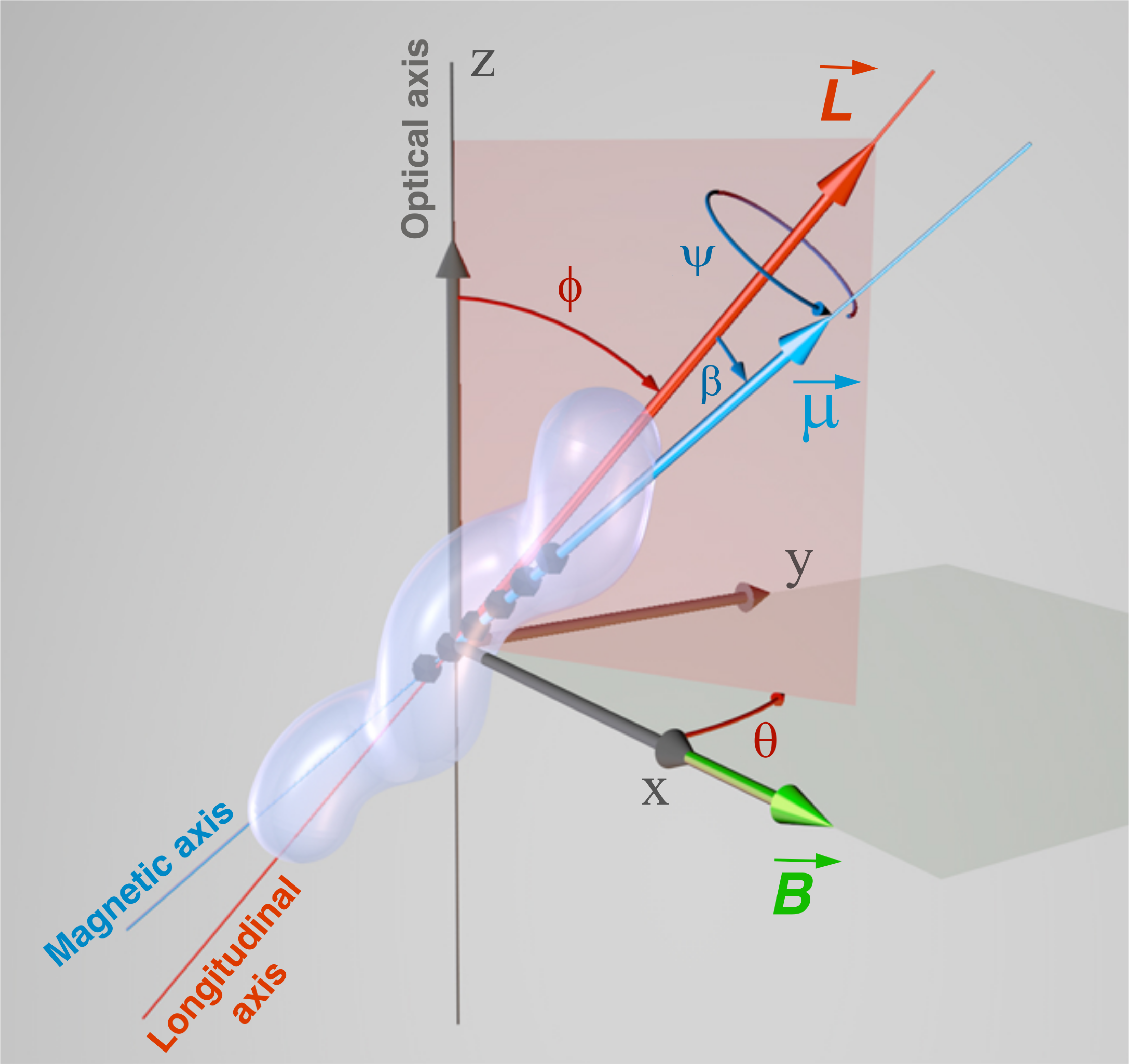
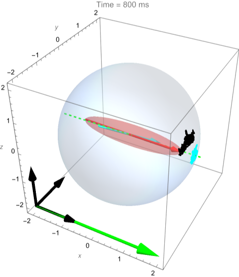
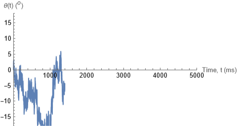
The following two figures are a projection of the particle and magnetic moment in the focal plane and a graph that shows the angles theta and psi as a function of time. The xlsx files needed to run the following animation are attached at the end of this post. Please make sure they are in the same directory of this notebook.
Trajectory to be animated
In[]:=
Filename="Simulation-Beta_20_degrees-B_5_mT-Repeat_#1-";ParticleXYZ=Drop[Import[NotebookDirectory[]<>Filename<>"L.xlsx"][[1]],1];MomentXYZ=Drop[Import[NotebookDirectory[]<>Filename<>"R.xlsx"][[1]],1];npoints=Length[ParticleXYZ];Angles=Table[{j,180/Pi*ArcCos[ParticleXYZ[[j,1]]/Sqrt[ParticleXYZ[[j,1]]^2+ParticleXYZ[[j,2]]^2]]*Sign[ParticleXYZ[[j,2]]]},{j,npoints}];MAngles=Table[{j,180/Pi*ArcCos[MomentXYZ[[j,1]]/Sqrt[MomentXYZ[[j,1]]^2+MomentXYZ[[j,2]]^2]]*Sign[MomentXYZ[[j,2]]]},{j,npoints}];
Parameters determining the look of the animation
In[]:=
(*Colors*)cparticle=Red;cmagneticmoment=Cyan;cmagneticfield=Green;(*Half-lengthofmagneticmoment*)MomentLength=1;(*Dimensionsoftheparticle-widthandhalf-length*)a=0.3;c=2;(*Plotdimension*)pdim=c*1.1;
Setting the plot axes
Fleche=Graphics3D[{cmagneticfield,Arrowheads[0.08],Arrow[Tube[{{-2,-2,-2},{2,-2,-2}},0.04]]}];Ligne=ListLinePlot3D[{{-pdim,0,0},{pdim,0,0}},PlotStyleDirective[cmagneticfield,Dashed]];Fx=Graphics3D[{Black,Arrowheads[0.06],Arrow[Tube[{{-2,-2,-2},{-0.5,-2,-2}},0.04]]}];Fy=Graphics3D[{Black,Arrowheads[0.06],Arrow[Tube[{{-2,-2,-2},{-2,-0.5,-2}},0.04]]}];Fz=Graphics3D[{Black,Arrowheads[0.06],Arrow[Tube[{{-2,-2,-2},{-2,-2,-0.5}},0.04]]}];(*Initializingtrajectories*)Traj=ListLinePlot3D[Take[ParticleXYZ*c,1],PlotStyleBlack,PlotRange{{-pdim,pdim},{-pdim,pdim},{-pdim,pdim}},BoxRatios{1,1,1},AxesLabel{x,y,z},PlotLabelRow[{"Time = ",0," ms"}]];MTraj=ListLinePlot3D[Take[MomentXYZ*c,1],PlotStylecmagneticmoment];ParticleAxis={};MagneticMoment={};Particle={};
In[]:=
(*Dynamic[Show[Particle,ParticleAxis,MagneticMoment,Traj,MTraj,Fleche,Fx,Fy,Fz]]*)Dynamic[Show[Traj,MTraj,Fleche,Ligne,Fx,Fy,Fz,ParticleAxis,MagneticMoment,Particle]]
Out[]=
Plot angular trajectory for θ
In[]:=
Angle=ListPlot[{},JoinedTrue,PlotRange{{0,npoints},{-90/5,90/5}},AxesLabel{"Time, t (ms)","θ(t) )"}];Dynamic[Angle]
o
(
Out[]=
In[]:=
Do[(*Trajectories*)Traj=ListLinePlot3D[Take[ParticleXYZ*c,n],PlotStyleBlack,PlotRange{{-pdim,pdim},{-pdim,pdim},{-pdim,pdim}},BoxRatios{1,1,1},AxesLabel{x,y,z},PlotLabelRow[{"Time = ",n-1," ms"}]];MTraj=ListLinePlot3D[Take[MomentXYZ*c,n],PlotStylecmagneticmoment];(*Ellipsoidofrevolution*)(*VectorL*)ParticleAxis=Graphics3D[{cparticle,Arrowheads[0.04],Arrow[Tube[{-c*ParticleXYZ[[n]],c*ParticleXYZ[[n]]},0.03]]}];(*Rotationawayfromtheopticalaxisandtowardsthemagneticaxis*)PhiL=ArcCos[ParticleXYZ[[n,3]]];r1=RotationTransform[-PhiL,{0,1,0}];(*Rotationinthefocalplane,awayfromthemagneticaxis*)ThetaL=ArcCos[ParticleXYZ[[n,1]]/Sqrt[ParticleXYZ[[n,1]]^2+ParticleXYZ[[n,2]]^2]]*Sign[ParticleXYZ[[n,2]]];r2=RotationTransform[-ThetaL,{0,0,1}];(*Changeofcoordinatefromthelabtotheparticlerefrential*)cprime=r1[r2[{x,y,z}]];(*Plotellipsoid*)Particle=ContourPlot3D[(cprime[[1]]/a)^2+(cprime[[2]]/a)^2+(cprime[[3]]/c)^2==1,{x,y,z}∈Ball[{0,0,0},2],ContourStyleDirective[Specularity[White,50],cparticle,Opacity[0.3]],Lighting"Neutral",Mesh->None,PlotPoints50(*ColorFunction(Hue[#4/4]&)*)(*,TicksNone*)];Angles=Table[{j,180/Pi*ArcCos[ParticleXYZ[[j,1]]/Sqrt[ParticleXYZ[[j,1]]^2+ParticleXYZ[[j,2]]^2]]*Sign[ParticleXYZ[[j,2]]]},{j,npoints}];(*Magneticmoment*)MagneticMoment=Graphics3D[{cmagneticmoment,Arrowheads[0.04],Arrow[Tube[{-MomentLength*MomentXYZ[[n]],MomentLength*MomentXYZ[[n]]},0.03]]}];(*Anglegraph*)Angle=ListPlot[Take[Angles,n],JoinedTrue,PlotRange{{0,npoints},{-90/5,90/5}},AxesLabel{"Time, t (ms)","θ(t) )"}];(*Finalgraph*)(*Print[n];*)(*Print[Show[Particle,MagneticMoment,Fleche,Fx,Fy,Fz]]*),{n,1,npoints,50}]
o
(
CITE THIS NOTEBOOK
CITE THIS NOTEBOOK
Propulsion matrix of the body of helical Magnetospirillum magneticum cells
by Cecile Fradin
Wolfram Community, STAFF PICKS, May 16 2023
https://community.wolfram.com/groups/-/m/t/2920289
by Cecile Fradin
Wolfram Community, STAFF PICKS, May 16 2023
https://community.wolfram.com/groups/-/m/t/2920289