A Single Photon, Single Angle Pair based Bell Type Experiment,
and
A study of 10 well known Quantum Operators with QuantumToMultiwaySystem
and
A study of 10 well known Quantum Operators with QuantumToMultiwaySystem
Abstract:
An initial Single Photon, Single Angle Pair based Bell type Experiment was conducted and completed as a proof of concept, sanity test, and infrastructure preparation for final publication. The possibility of such an experiment emerged after generating 6 Bell-Aspect type diagrams along with 6 absolute value diagrams on a single page shown below. At first there was some doubt that it would be possible without a ‘real’ lab with an expensive SPDC entangled correlated source and automated time stamped single photon counters. However, after some preliminary test results, the experiment looked possible and was executed in a home optics setup with a simple power meter and an ordinary He-Neon laser.The intent now is to drive up Sigma and turn this into a published experiment.
In parallel to the above experiment, and motivated by two recent Bell type entanglement of entanglement experiments which ‘proved’ that quantum mechanics requires complex numbers, preparation of the mathematical infrastructure for single photon based experiments of this type were made. As a follow-on to the completion of this experiment, the hope is to be able to do these single photon type entanglement of entanglement experiments, and show the value of the Mathematica QuantumToMultiwaySystem generated Multiway Diagrams in exploring the subtler aspects of Quantum Mechanics. For this part of the project, dozens of related Multiway diagrams were generated using 10 common quantum operators entangled with single pair Bell measurements . (Here, again, the value is to show that the big picture with a wide overview generates new possibilities.)
Section1: 6 Bell-Aspect diagrams (and 6 absolute value graphs) give a hint of what might be possible:
Section1: 6 Bell-Aspect diagrams (and 6 absolute value graphs) give a hint of what might be possible:
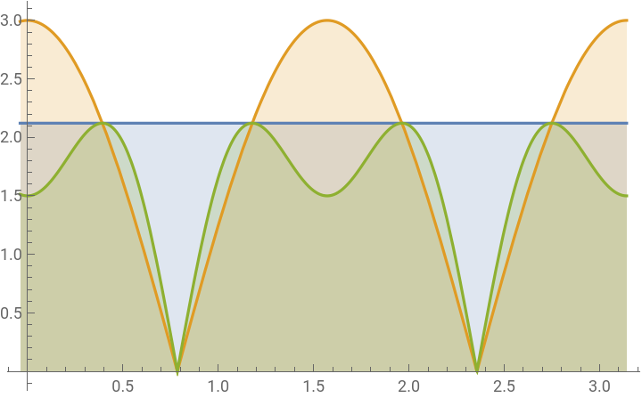
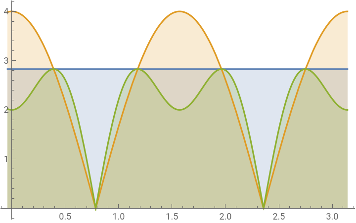
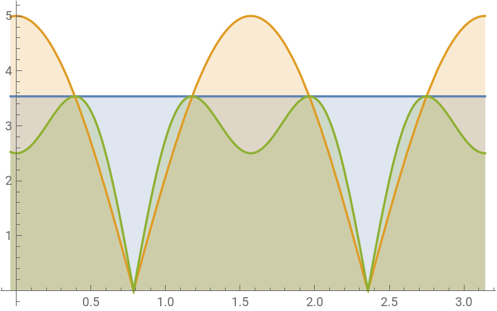
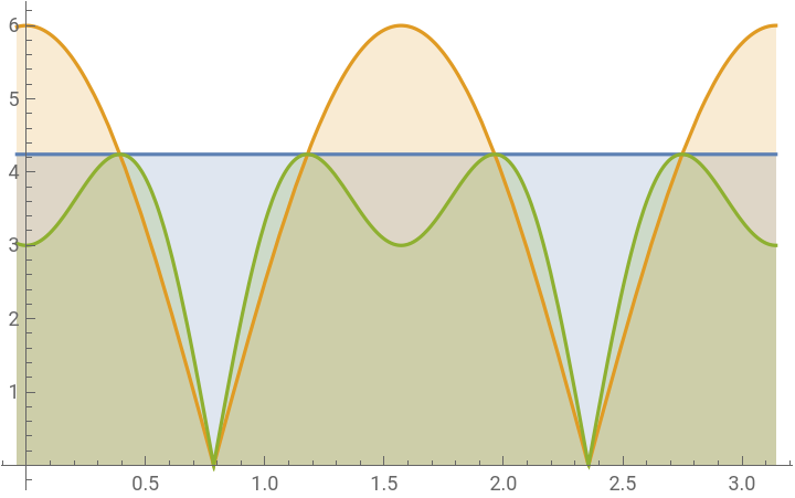
Below are the Bell-Aspect diagrams from 1 to 6 angle pairs, as well as their Absolute values. The top left position on each graph in the 2nd line from 1 to 6 indicates the number of pairs.(View the 2nd row of graphs to see the 5 on the top left.) The = (The green values on the left are the traditional 4 pair Bell inequality values.)
light orange background
indicates the generalized Bell-Aspect equations below. The graphic unification below brings out their overall structure.The orange curves in each graph represent the simple quantum mechanical cases. The green curves are the Bell-Aspect diagrams.The top green-blue horizontal line in each graph represents the maximum of the Aspect curves and correspond to: ,,,,,
1
2
2
2
3
2
4
2
5
2
6
2
,,,3
1
2
2
,3
2
2
,2
5
2
2
TablePlot,n(Cos[2k]),(3Cos[2k]-Cos[3(2k)]),π,Filling->Bottom,{n,{1,2,3,4,5,6}}
n
2
n
4
,k,-0.1π
8
Out[]=
,
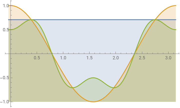
,
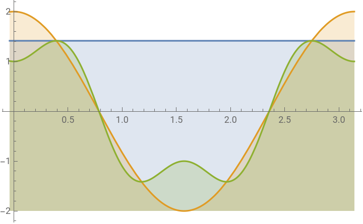
,
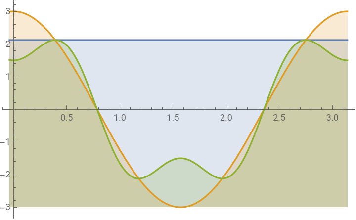
,
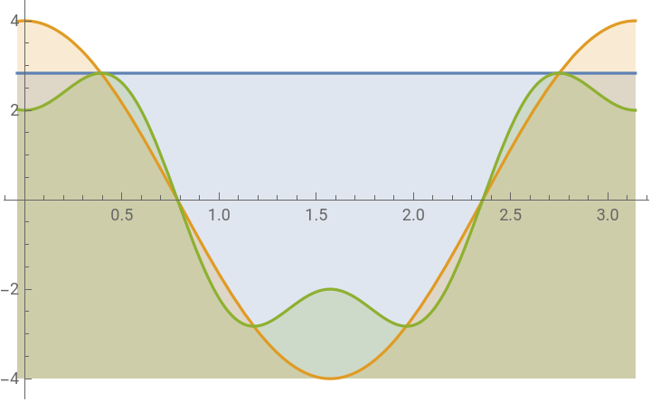
,
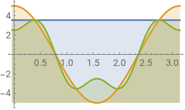
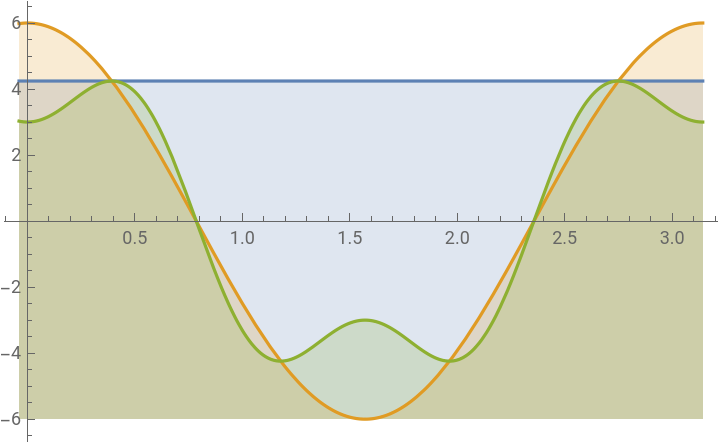
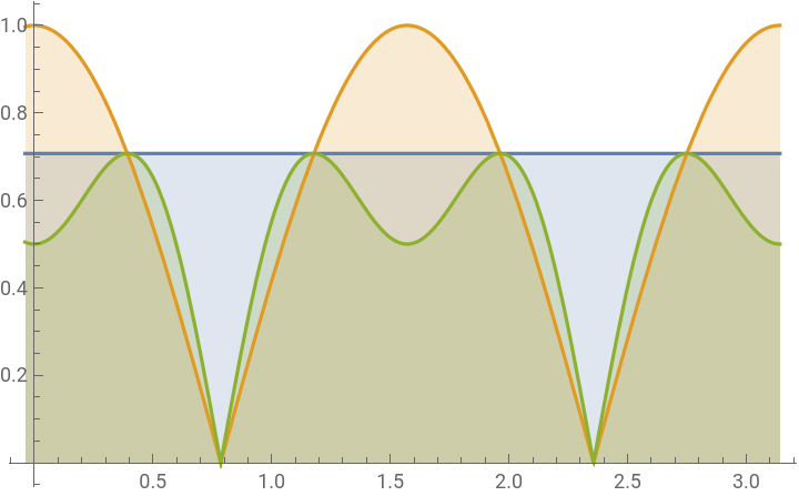
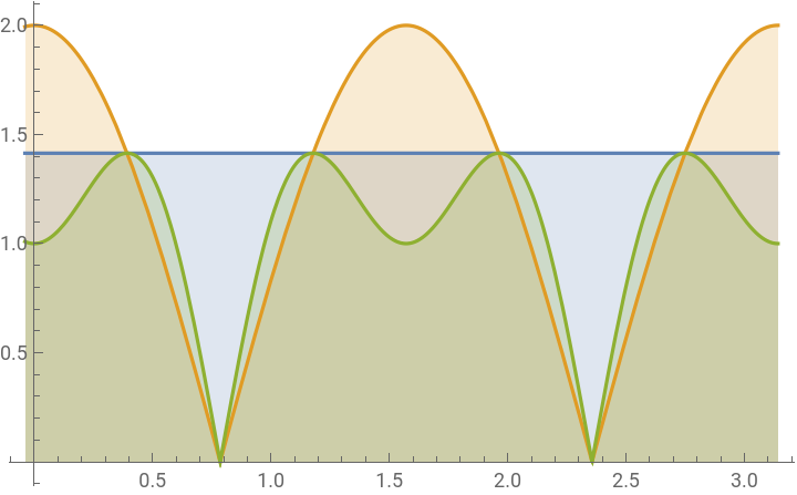
The Absolute Values of all six cases is generated below. We will ultimately find out that the orange absolute value of the quantum cases below are key:
In[]:=
TablePlot,Abs[n(Cos[2k])],,π,Filling->Bottom,{n,{1,2,3,4,5,6}}
n
2
Abs(3Cos[2k]-Cos[3(2k)])
n
4
,k,-0.1π
8
Out[]=
,
,
,
,
,
Below is the superimposition of all the graphs above, with the red and purple lines showing the absolute value action which have been compressed. (Double click tab on right to view.)
TablePlot,n(Cos[2k]),Abs[n(Cos[2k])],(3Cos[2k]-Cos[3(2k)]),π,Filling->Axis,{n,{1,2,3,4,5,6}}
n
2
n
4
,
Abs(3Cos[2k]-Cos[3(2k)])
n
4
,k,-0.1π
8
The KEY POINT: Perform the single photon, single angle pair Bell experiment.The implications of the graphs above is that the results of the Bell experiment have the same form for any number of pairs. This immediately hints at the possibility of doing a simple experiment with a single pair. In physics, a single pair experiment brings to mind the single photon two slit experiment, where one photon (or one particle) interference creates a non-local entangled result. have stated in their book on Quantum Entanglement that interference and entanglement are fundamentally equivalent and are at the same level. We shall see that the experiment below is the very experiment missing from the numerous beautiful examples in his book.
FJDuarte&TS
1
Taylor
Section2: The Single Photon, Single Angle Pair Bell experiment
Section2: The Single Photon, Single Angle Pair Bell experiment
Before we dive into the experiment, it is important to mention that a single, double, and triple pair Bell type experiment, were suggested in the original paper in 1969 by Clauser, Horne, Shimony and Holt in Physical Review Letters, Volume 23, Number 15, 13 October 1969. Below, a relevant piece of that information suggesting the single, double, triple forms of a Bell experiment:
2
CHSH

In a good history by M Frank of some entanglement research by Wu & Shaknov, where reference to Clauser is made, is in the April 2023 issue of Scientific American, (as well as the article about research on how imaginary numbers are needed in Quantum Mechanics.)
Below is the simple experiment set up, data and results.
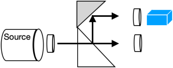
1. The He-Ne laser source has some optics in front of it to reduce the intensity to protect the sensitive laser power detector ( 2 film polarizers at 45 degrees) and a polarizer set at 0 degrees.This insured that most photons emerging from the laser is linearly polarized vertically.
2. A beam splitter: Most beam splitters are not 50-50 and different techniques must be used to equalize the beams. This is one area where future improvements will be possible in this experiment. One technique is to use continuous diffusion filters to make sure both beams are starting with the same intensity. One beam goes straight through a polarizer which remains at vertical throughout the whole experiment.
3. A 45 degree mirror is used to send the 2nd beam into the 2nd polarizer which is rotated in 20 degree increments and measured by a laser power meter.
This is done in the dark with little flash lights to avoid errors from reading lights and turning the polarizers. Each time a reading of the laser power meter is made, it takes a few seconds for the power meter to settle down. Care is taken not to let stray recording light reach the power meter.
4. Below the horizontal line at the end of this section are 19 angle sets of data, one for each angle with 14 readings. The Mean and Standard Deviation (∑) is calculated for each set.
5. Here, each of the 19 angle sets are assembled in to two groups, the Means (set), and the Standard Deviation (std); to see the date, go to the horizontal line at the end of this report, where the data is organized. (The 4 lines below are the result of that data organization.)
5. Here, each of the 19 angle sets are assembled in to two groups, the Means (set), and the Standard Deviation (std); to see the date, go to the horizontal line at the end of this report, where the data is organized. (The 4 lines below are the result of that data organization.)
In[]:=
set={set0,set20,set40,set60,set80,set100,set120,set140,set160,set180,set200,set220,set240,set260,set280,set300,set320,set340,set360}
Out[]=
{set0,set20,set40,set60,set80,set100,set120,set140,set160,set180,set200,set220,set240,set260,set280,set300,set320,set340,set360}
In[]:=
std={std0,std20,std40,std60,std80,std100,std120,std140,std160,std180,std200,std220,std240,std260,std280,std300,std320,std340,std360}
Out[]=
{std0,std20,std40,std60,std80,std100,std120,std140,std160,std180,std200,std220,std240,std260,std280,std300,std320,std340,std360}
6. Nineteen (19) data points in set[[n]], which are associated with 19 angles from 0to ( 0 to π in 20 degree increments) are List Plotted below. Ideally, the data point for angle 0 and angle 360, should be that same.This was done in two cycles: one from 0 to π and one from back to 0 in 20 degree increments. However, physically in terms of the polarizer is 180 degrees. However 360 degrees is the same position as 0 degrees. Despite the low standard deviation values, especially at the lowest points of the graph corresponding close to the sensitivity limits of the power meter, remarkably, the maximum dips are close to (between the 5th and 6th data points) and (between the 13th and 14th data points) and lie right above the angle ticks. Much more care is necessary to equalize the beams at zero and 180 degrees to make the results correspond more closely to the calculated graphs.(Caution; each of the angles at the bottom must be run one by one to run a copy of this summary on a another computer.)
π
18
18
π
18
8π
8
8π
8
π
4
3π
4
In[]:=
ShowPlot,,π,Filling->Bottom,ListPlotAssociationThreadTablen,{n,0,18},Table,{n,1,19},Ticks->,Pi4,3Pi8,Pi2,5Pi8,6Pi8,7Pi8,Pi,,1
2
2
Abs[Cos[2k]]
,k,-0.1π
8
π
18
set[[n]]
set0
π
8
2
2
Out[]=
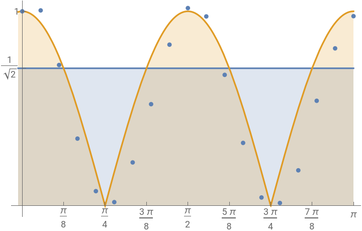
7. Below, the Standard Deviation of all the standard deviations is calculated to be 0.608; this ∑ is a not a value that is acceptable. However, for this proof of concept, sanity test without a single photon counter, it shows that there is hope. It is interesting to note that the and ticks at the lowest dips in the graph lie remarkably close to where they belong. Also, the overall shape of the curve is Quantum like, and the individual Sigma values listed below the graph approach 1.95. One way to immediately increase the Standard Deviation would be to use neutral density filters to even out beam intensities emerging from the beam splitters. Also, the experiment should be done both in right hand and left hand configurations to average out errors.
π
4
3π
4
In[]:=
StandardDeviation[std]
Out[]=
0.608385
8. We now plot the data with the Bell Inequality and Quantum Mechanics curves:
Single photon, single angle pair Aspect Graph showing Bell Inequality Violations above the blue line:
Single photon, single angle pair Aspect Graph showing Bell Inequality Violations above the blue line:
July 10th Measurements: Mathematica’s Standard Deviation function was used to confirm the Sigma level of the experiment which reached 1.95 for 200 degrees.
The Summary of the Means and Sigma for all angles are listed below:
{ angle, mean, Sigma}
{ 0, 63.5286, 1.64944 }
{. 20, 63.8244, 1.64944 }
{ 40, 45.9933, 1.43848 }
{ 60, 21.95, 0.19115 }
{ 80, 4.79286, 1.01335 }
{ 100, 1.20714, 0.154244}
{ 120, 14.1714, 0.255489}
{ 140, 33.2, 0.885785}
{ 160, 52.6357, 0.381509}
{ 180, 64.5857, 1.92947 }
{ 200, 61.8571, 1.95043 } BEST
{ 220, 42.7733, 0.843857}
{ 240, 20.5467, 0.747249}
{ 260, 2.72143, 1.62726 }
{ 280, 0.923077, 0.227866}
{ 300, 11.5929, 0.535601}
{ 320, 34.3077, 1.19824 }
{ 340, 51.4286, 0.895757}
{ 360, 61.9429, 0.09759 }
Section 3: Using QuantumToMultiwaySystem to generate Multiway diagrams in some entanglement of entanglement simulations between a two angle Bell measurements, and a study of 10 Quantum Operators
(A request: please send more operators)
Section 3: Using QuantumToMultiwaySystem to generate Multiway diagrams in some entanglement of entanglement simulations between a two angle Bell measurements, and a study of 10 Quantum Operators
(A request: please send more operators)
(A request: please send more operators)
Since the Hadamard and modified Hadamard operators are similar to the Pauli operators above, we generate them here for easy comparison.
The entanglement is now turned on; as above with the Pauli operators, we generate 10 = { (4 x 3 ) -2 } unique non-duplicated diagrams because two t = 1 cases are duplicates.
The first and second rows for t =2 (2nd column) look similar but are different, especially in the bottom left.
On both wave functions;
On three:
On four targets:
The Swap Gate works on the following set: { {{1,0,1,0}}, {{1,1,0,0}}, {{1,0,1,1}}, {{1,1,0,1}}, {{1,0,1,1}}
Another different 5 targets:
On both wave functions;
On three:
On four targets:
The Swap Gate works on the following set: { {{1,0,1,0}}, {{1,1,0,0}}, {{1,0,1,1}}, {{1,1,0,1}}, {{1,0,1,1}}
Another different 5 targets:
Swap Gate with EvolutionEventsGraphStructure; a half wave plate on the 2nd term does wonders and completes the series at t = 6:
The bottom of the graph below for this EvolutionGraph clearly shows why it is called the Swap Operator:
Next we do the root-SWAP operator; the 2 values in the first and last operator lines is especially interesting:
The completion diagram of this looks like the completion diagram of the root-NOT operator:
The example below for t = 2, 3,and 4 correspond to the root-NOT operator diagrams.
The Toffoli Gate: we use the QuantumToMultiwaySystem Function Repository example of a starting point:
https://resources.wolframcloud.com/FunctionRepository/resources/QuantumToMultiwaySystem
https://resources.wolframcloud.com/FunctionRepository/resources/QuantumToMultiwaySystem
Toffoli gate with EvolutionEventsGraphStructure and a half wave plate header on the first term:
Toffoli gate
The FredkinGate; the last 3 operators out of 8 replace 2 diagonal terms with 2 off diagonal terms:
Form 8D to 5D:
The CNOT gate: The off diagonal terms are in the bottom right corner:
The CNOT gate with 2 imaginary ‘kickers:’
Below is the data set for The Single Photon, Single Angle Pair Bell experiment
0 degrees
20 degrees
40 degrees
60 degrees
80 degrees
100 degrees
120 degrees
140 degrees
160 degrees
180 degrees
200 degrees
220 degrees
240 degrees
260 degrees
280 degrees
300 degrees
320 degrees
340 degrees
360 degrees
In Appreciation to:
Takeshi Yoneyama, who pushed me to study quantum mechanics again,
to my mentors, Shivam Sawarn, Hatem Elshatlawy, Xerxes Arsiwalla,
to Mark Greenberg who enabled multiple sets of diagrams from a single equation,
to Nikolay Murzin for getting normalized wave functions appear in QuantumToMultiwaySystem, and to Johnathan Gorard who created it,
to all the support people who made this Summer School possible,
to Stephen Wolfram who created the Physics Project and the Summer Schools, and continues to enhance this wonderful experience for so many people from around the world,
and last but not least, Patricia, my Lab Manager.
CITE THIS NOTEBOOK
CITE THIS NOTEBOOK
Single photon, single angle pair bell experiment
by Mark Merner
Wolfram Community, STAFF PICKS, July 13, 2023
https://community.wolfram.com/groups/-/m/t/2960649
by Mark Merner
Wolfram Community, STAFF PICKS, July 13, 2023
https://community.wolfram.com/groups/-/m/t/2960649