Wolfram Cloud Document

The Arctic sea-ice cap at the end of every melt season, 1979–2024, seen from above the North Pole. Re-coloured from NSIDC monthly concentration GeoTIFFs (polar-stereographic). September extent has fallen from ~7.0 to ~4.3 million km² — roughly a 40% loss in four decades.

The NSIDC Sea Ice Index gives daily sea-ice extent for both polar regions from late 1978 to today. Here the daily series is separated into a slowly-varying long-term trend, a deterministic annual cycle (a short Fourier harmonic series), and a residual. Removing the predictable annual march of freeze and melt sharpens one question: after the seasonal cycle is taken out, in which years does the ice behave unlike its neighbours? A change-point detector flags an apparent Arctic break near 2003–04, but a model comparison shows the Arctic decline is better described as a smooth gradual trend than as discrete regimes; the Antarctic instead rose to a ~2014 high and then fell, a swing a straight line cannot capture but a smooth curve can. Once the trend is removed, no significant change-point survives in the residual — the trend already carries the low-frequency story — yet individual years (Arctic 2007 and 2012, Antarctic 2014, 2016, 2023) stand out as notable — though, as §15 shows, not field-significant once multiple comparisons and autocorrelation are accounted for. Everything below is pure Wolfram Language.

Setup — load the companion package

Every analysis and figure below is produced by the companion package arctic_seaice.wl, attached to this post. Put it next to the notebook and load it. The package fetches the NSIDC daily extent directly from the web (and caches it), so an internet connection is needed the first time; thereafter everything runs offline. Each code cell shows the exact call — evaluate it to reproduce the figure above it.

SetDirectory[NotebookDirectory[]];<<arctic_seaice.wl(*oneassociationholdsthewholedecompositionforahemisphere:*)dec=Decomposition["north","K"->4,"TrendSigmaDays"->730.];Keys[dec]

The September ice-cap animation at the top is itself reproducible — SeptemberIceCapAnimation[Range[1979, 2024]] downloads the September concentration GeoTIFFs and renders the frames (slow; the result is embedded above).

1. The data: NSIDC daily sea-ice extent

Sea-ice extent is the total area of ocean with at least 15% ice concentration, in millions of square kilometres. The NSIDC Sea Ice Index v4.0 publishes it daily for each hemisphere. The record starts 26 October 1978; it is every-other-day until mid-1987 and daily thereafter, with one documented multi-week gap at the 1987–88 satellite transition. We fetch the CSV directly and place the values on a regular daily grid by linear interpolation across the short gaps.

base = https://noaadata.apps.nsidc.org/NOAA/G02135;
N_daily = base <> /north/daily/data/N_seaice_extent_daily_v4.0.csv;
S_daily = base <> /south/daily/data/S_seaice_extent_daily_v4.0.csv;

The raw Arctic series, with the long-term trend (a 2-year edge-renormalised Gaussian low-pass of the deseasonalised series) overlaid:

ExtentTrendPlot["north"]

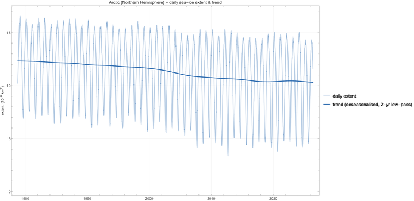
Daily Arctic sea-ice extent (light) and its long-term trend (dark). The annual cycle dominates the raw series; the trend is what is left once it is averaged out.

2. Decomposition: trend + annual harmonics + residual

We use the classic additive decomposition

extent(t)=trend(t)+seasonal(t)+residual(t)

estimated in two passes. First the seasonal component is the periodic part of a harmonic regression of extent on a linear term plus

annual harmonics,

seasonal(t)=

∑

k=1

[

cos(2πkt)+

sin(2πkt)]

with

= 4 (the fundamental plus three overtones — enough to capture the asymmetry between the slow autumn freeze-up and the faster summer melt). The linear term only de-biases the harmonics and is then discarded. Subtracting the seasonal part gives the deseasonalised anomaly; smoothing that with a 2-year Gaussian low-pass gives the trend; and the residual is whatever remains.

The heart of the method (this is what HarmonicSeasonal in the package does):

HarmonicSeasonal[t_,y_,K_]:=Module[{design,c},design=Function[ti,Join[{1.,ti},Flatten@Table[{Cos[2Pikti],Sin[2Pikti]},{k,K}]]]/@t;c=LeastSquares[design,y];(design.c)-(c[[1]]+c[[2]]t)(*periodicpartonly*)]

For the Arctic the trend and seasonal cycle reconstruct the daily extent essentially exactly and explain 98.5% of its variance. Reproduce the four-panel decomposition with:

dec=Decomposition["north","K"->4,"TrendSigmaDays"->730.];{dec["varExplained"],dec["seasonalAmp"],dec["residualSD"]}DecompositionPlot["north"]

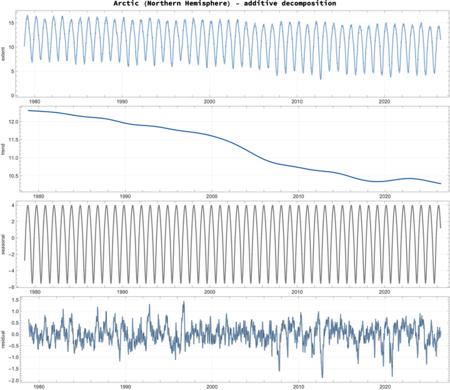
Additive decomposition of Arctic daily extent. Top to bottom: the data, the long-term trend, the harmonic annual cycle, and the residual. Note the residual's growing scatter and the isolated deep excursions after ~2000.

3. The seasonal cycle as a harmonic series

The fitted annual cycle has a peak-to-trough amplitude of 9.5 × 10⁶ km² in the Arctic. Its shape is not a pure sinusoid — the autumn re-freeze is gentler than the spring/summer melt — which is exactly why more than one harmonic is needed.

SeasonalPlot["north"]

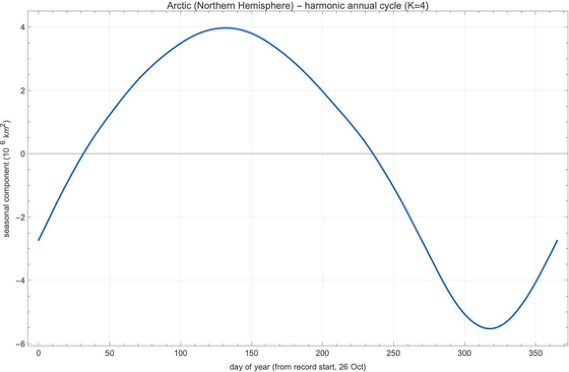
The Arctic annual cycle recovered as a K=4 harmonic series (anomaly form, annual mean removed).

4. Change-point detection: regime shifts after seasonal removal

Change-point detection is run at calendar-year resolution using binary segmentation (Gaussian SSE cost, BIC penalty) and a CUSUM statistic. An important honesty note up front: annual averaging does not make the values independent — the annual-mean anomaly is itself strongly autocorrelated (lag-1 r ≈ 0.94 in the Arctic). A permutation null that shuffles years therefore badly understates uncertainty, so the locations below are descriptive and their significance is assessed honestly in §15 (an AR(1) surrogate gives p ≈ 0.06, i.e. not significant).

The CUSUM statistic (CUSUM) and a permutation test — kept only to show why it is wrong here:

CUSUM[x_]:=Accumulate[x-Mean[x]];CUSUMTest[x_,nperm_:5000]:=With[{s=Max@Abs@CUSUM[x]},(*permutationnull:INVALIDforautocorrelatedx*)N[(1+Count[Table[Max@Abs@CUSUM[RandomSample[x]],{nperm}],r_/;r>=s])/(nperm+1)]]

Applied to the deseasonalised anomaly (extent − seasonal, trend retained), binary segmentation puts a single Arctic break around 2004 (11.89  10.54 × 10⁶ km²). But a mean-shift detector can only produce flat plateaus, so on a smoothly varying series it is forced to fake steps. The honest test is not "line vs step" but a three-way contest: a straight line, a smooth curve (here a cubic), and the piecewise-constant regime model. A line fitting badly does not make steps right — a curve might fit just as well with no abrupt change at all.

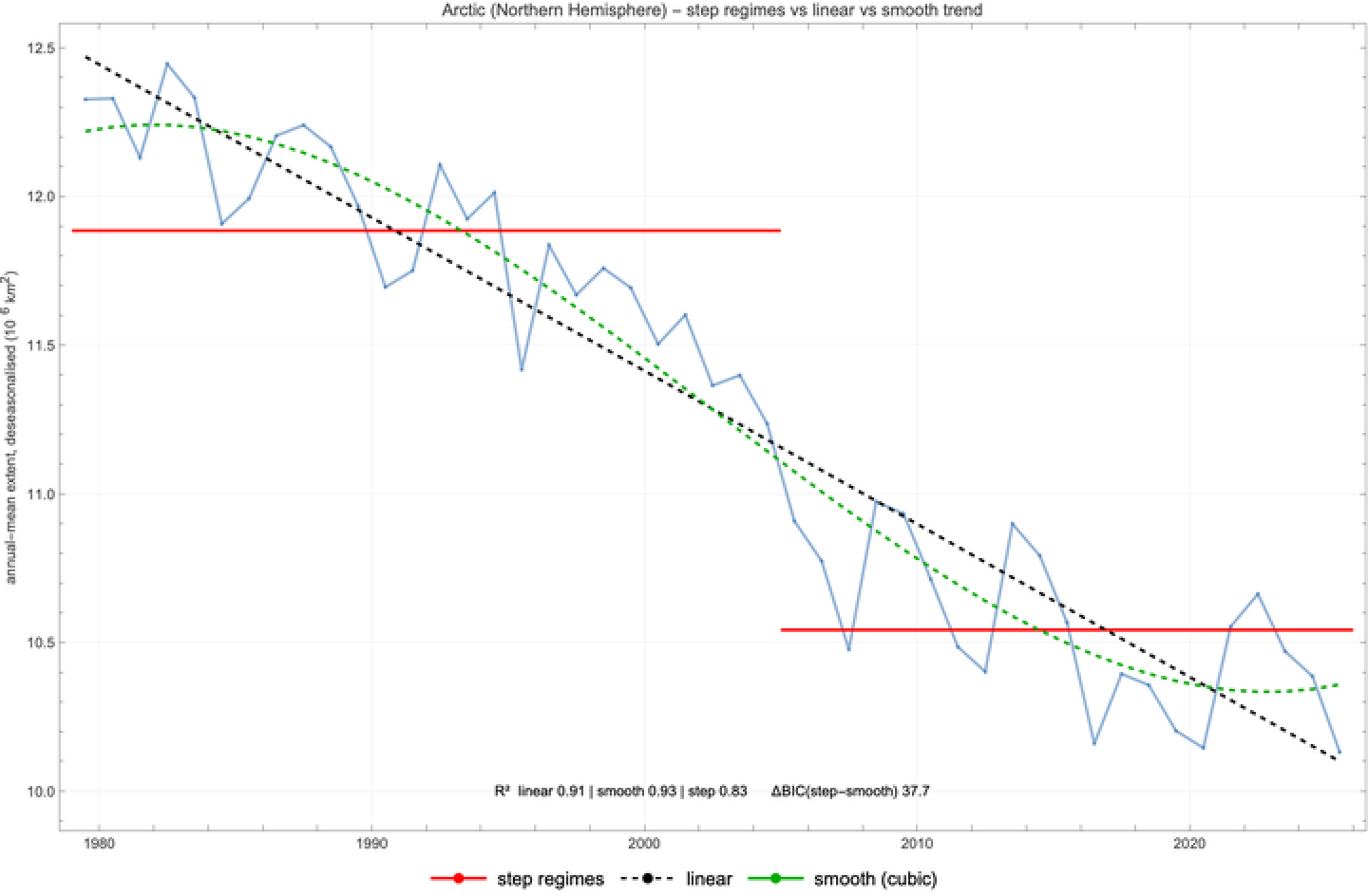
Annual-mean deseasonalised extent with three competing fits: step regimes (red), a straight line (dashed black), and a smooth cubic (green). Lower BIC = better; ΔBIC > ~6 is usually called decisive.

Arctic: a smooth gradual decline wins outright. The straight line already explains 91% of the variance and a gentle cubic curve nudges that to 93%; the two-plateau model is far worse (R² = 0.83, and its BIC is ~38 higher than the smooth fit). The decline is continuous — the "regime shift" is an artefact of forcing a piecewise-constant fit, which is why the smooth trend of §2 (and the stationary residual of §5) is the right description.

Antarctic: genuinely different, but the conclusion is more careful than "it needs steps". The series rose to a ~2014 high and then fell, so a straight line is useless (R² = 0.03) — but that argues for a curve, not necessarily abrupt shifts. A smooth cubic captures the rise-and-fall well (R² = 0.52), and the step model is only marginally better (R² = 0.63, ΔBIC ≈ 8). That margin is "positive" by the book, but it is inflated by the strong year-to-year autocorrelation (the effective sample is far smaller than 47), and a more flexible smoother would close most of it. With this much data we cannot cleanly separate "two abrupt regime shifts" from "one fast but continuous swing"; physically, the rapid 2016 drop is the most step-like feature, while the 2007 rise is gradual. The defensible summary is that both hemispheres are best read as smooth trends — monotonic in the Arctic, a hump in the Antarctic — and a discrete "regime" picture is a possible, not an established, alternative.

5. The residual is (nearly) stationary

What happens if we also remove the trend and run the same detector on the residual? Nothing significant (AR(1)-surrogate p = 0.98 Arctic, 0.84 Antarctic). Note this is partly circular — the trend is a 2-year low-pass of this very series, so removing it must leave no multi-year structure (a point made fully in §15). It is still a useful consistency check: the residual is genuinely near-white (lag-1 r = 0.03), so the apparent §4 step really lives in the trend itself rather than being an abrupt jump on top of it.

Arctic annual-mean residual (trend and season both removed). No mean change-point is significant — a check that the decomposition has done its job.

The one thing the residual does show is changing year-to-year volatility: within-year residual spread quadruples from quiet years (~0.2) to the most eventful ones (~0.8), with sharp peaks in 1996, 2007, 2012 and 2020.

Within-year standard deviation of the Arctic residual. The tall years are those in which the ice departed sharply from its trend+season expectation at sub-annual scale.

6. Which years stand out after seasonal removal?

Standardised Arctic annual-mean residual. Bars beyond the dashed ±1.96 lines cross the nominal 5% line (1995, 2007) — but see §15: this is a screening threshold, not a multiple-comparison-corrected test.

Interestingly, the record-shattering melt year 2012 is not flagged on the annual mean — its crash was concentrated in late summer, so it instead dominates the volatility plot above. The single most extreme daily residual in the whole Arctic record is indeed 30 September 2012, 1.90 × 10⁶ km² below the trend+season expectation — the method rediscovers the famous 2012 minimum on its own.

7. The Antarctic contrast

The Southern Hemisphere tells a different and more dramatic story. Its annual-mean anomaly rises to a high plateau (break around 2007), then collapses after 2015 (12.20 → 10.88, CUSUM break 2015, p < 0.001) — the abrupt Antarctic decline that has preoccupied polar scientists since 2016.

Antarctic annual-mean deseasonalised extent with its three mean regimes. The post-2015 drop and the record-low 2023 are clearly visible.

The unusual-year scan flags Antarctic 2014 as a record high, and 2017 and 2023 as record lows; the most extreme single day is 14 December 2016, 2.22 × 10⁶ km² below expectation.

8. A deepening: the seasonal cycle is amplifying

Fitting an independent linear trend to each calendar month exposes what the annual-mean trend hides. In the Arctic every month is declining (all p < 0.001), but the late-summer and autumn months are falling roughly twice as fast as spring: October −0.78, September −0.76 and August −0.71 versus May −0.31 (10⁶ km² per decade). The summer ice is vanishing faster than the winter ice, so the peak-to-trough seasonal amplitude is growing at +0.38 × 10⁶ km²/decade (p < 0.001).

Arctic decadal trend by calendar month. The deep summer/autumn bars are the ice-free-season expansion.

Splitting the year into its extremes confirms it: the summer minimum is dropping at −0.75 × 10⁶ km²/decade while the winter maximum falls only −0.40 × 10⁶ km²/decade (both p < 0.001). Yet the calendar of the cycle is essentially fixed: the dates of the minimum (~13 Sep) and maximum (~10 Mar) and the melt-season length (~188 days) show no significant drift. The Arctic cycle has deepened, not shifted.

Arctic annual maximum (top) and minimum (bottom) extent. The widening gap is the growing amplitude; the steep 2012 dip is the record minimum.

9. A deepening: how much memory does the residual have?

Treating the daily residual as a time series, its periodogram closely follows the spectrum of a first-order autoregressive (red-noise) process. Fitting AR(1) gives an anomaly e-folding memory of ~106 days (~3.5 months) in the Arctic and ~182 days (~6 months) in the Antarctic — the Antarctic remembers a perturbation about twice as long. Two features stand out above the red-noise background: a sharp line at exactly 1 cycle/year (the fingerprint of the amplifying seasonal cycle that a stationary harmonic cannot absorb), and suppressed power at multi-year periods (removed with the trend).

Arctic residual periodogram (points) against the fitted AR(1) red-noise spectrum (grey) and its 95% level (red). Annual line at 1 cycle/yr; low frequencies fall below the background because the trend absorbed them.

10. A deepening: anomaly reemergence

Arctic anomaly memory map: correlation between an anomaly in each start month (rows) and the anomaly a given number of months later (columns). Off-diagonal warm bands are the reemergence signal.

11. Global sea ice and the two hemispheres

Adding the two hemispheres gives the global total. Because the Arctic peaks in March and the Antarctic in September, the two annual cycles are nearly in anti-phase, so the global total swings less than either pole alone (it ranges ~15.7–28.3 × 10⁶ km²). The long-term global trend was gently downward for decades and then fell sharply after about 2015 — the combined signature of the steady Arctic decline and the abrupt Antarctic drop, which together produced the record-low global sea ice of the mid-2020s. (Note: this is extent — area with ≥15% concentration — not concentration-weighted area.)

Global sea-ice extent (grey) with the Arctic and Antarctic contributions and the global trend (black). The post-2015 downturn is the recent record-low global ice.

12. Do the two poles move together?

Left: North vs South monthly anomalies (no relationship). Right: their cross-correlation by lag stays near zero throughout.

13. How the September ice-cap animation is built

The opening animation is made entirely in Wolfram Language from NSIDC monthly concentration GeoTIFFs (north polar-stereographic, 304×448 @ 25 km). For each year the colour-rendered tile is re-coloured pixel-by-pixel into a "view from space" palette — grey land, deep-blue ocean, luminous ice — the September pole-hole is filled with ice, the frame is cropped to a pole-centred square and given a circular vignette, and the year + extent are overlaid. SeptemberIceCapFrame builds one frame and SeptemberIceCapAnimation assembles them; the colour map is just:

Render the whole thing (downloads the September GeoTIFFs the first time, then renders ~46 frames):

14. Harmonics on the whole sphere: the global temperature field

The same harmonic thinking generalises from one time series to the entire planet. Take the NCEP/NCAR surface-air-temperature climatology (12 monthly maps on a 2.5° grid) and ask two questions: how big is the annual cycle at each point, and how is the mean field organised across the sphere?

Fitting a one-cycle harmonic in time at every grid point gives the amplitude of the annual march of temperature. It is tiny over the tropical oceans (a degree or two) and enormous over the high-latitude continents — up to ~27°C over Siberia — because land has little thermal inertia. This is exactly the same calculation as the sea-ice seasonal cycle, done pixel by pixel.

Amplitude of the annual temperature cycle. Large over continental interiors and the poles, small over oceans and the tropics.

Angular power spectrum of annual-mean temperature (ℓ ≥ 1). Degree 2 — the pole-to-equator gradient — dominates; power falls off toward high degree.

Annual-mean temperature (top) and its spherical-harmonic reconstructions. ℓ ≤ 2 is the equator-pole gradient; ℓ ≤ 6 adds the land-sea pattern.

And the field textured onto a globe — harmonics on the actual surface of the Earth. This one is a live 3-D object: drag to rotate it.

15. What the data actually support — uncertainty, assumptions, pitfalls

A decomposition pipeline can manufacture structure, so it is worth stating plainly which conclusions survive scrutiny and which are artefacts of the method. The points below were sharpened by two adversarial reviews (a statistician's critique and an external model's). The recurring lesson: serial correlation quietly invalidates the naive significance tests, so several headline p-values are not what they seem.

Autocorrelation deflates the change-point "significance"

The "stationary residual" check is partly circular

Because the trend is a 2-year low-pass of the very series being analysed, removing it necessarily leaves no multi-year structure behind — so "no change-point survives in the residual" (§5) is partly definitional, not independent confirmation. It is still a useful consistency check (the residual is genuinely near-white: lag-1 r = 0.03, nₑ ≈ 45), and the headline decline magnitude is robust to the bandwidth (−2.2 to −1.9 × 10⁶ km² for a 1–4-year filter), but it should not be sold as proof that the decomposition is "correct".

Trends: with honest confidence intervals, the amplification survives

"Unusual years" are screening flags, not field-significant outliers

Testing all 47 years at the 5% level, about 2.4 false flags are expected by chance — and 2 (Arctic) / 3 (Antarctic) are flagged. The most extreme single year reaches |z| = 2.16 (Arctic), below the familywise-95 threshold of 3.10 from an AR(1) null (familywise p = 0.82). So 1995/2007/2012 are best called notable years — consistent with the documented record events — but they are not statistically unusual once multiple comparisons and autocorrelation are accounted for.

A fixed seasonal cycle, a reddened daily spectrum

The seasonal model is a stationary harmonic, yet §8 shows the amplitude is growing — so the residual carries a residual 1-cycle/yr line (§9) and is not perfectly stationary. The memory timescales (~3.5 / 6 months) are therefore order-of-magnitude figures, not uncertainty-bounded estimates; the early every-other-day record and the interpolated 1987–88 gap further redden the daily periodogram. A time-varying-amplitude harmonic would tighten this.

The spherical-harmonic transform is validated — at low degree

Reassuringly, the naive sin-latitude quadrature on the 2.5° grid is accurate: the discrete orthogonality leakage is below 0.003 and the Parseval ratio is 0.96 (ℓ ≤ 4) / 0.98 (ℓ ≤ 8), so the degree-2 dominance and the low-degree spectrum are trustworthy. We do not over-interpret the high-ℓ tail, which is grid-dependent.

Bottom line: deducible vs. model-dependent

Supported by the data: the large seasonal cycle; a gradual Arctic multidecadal decline of ~2 × 10⁶ km² (interval-bounded, bandwidth-robust); seasonal amplification (summer ~2× winter); an Antarctic that rose then fell (a straight line fails); and degree-2 (equator–pole) dominance of the global temperature field.

Not established by this analysis: discrete "regime shifts" as significant events (they vanish under an AR(1) null); specific change-point years as genuine breaks rather than a description of a smooth trend; individual "statistically unusual" years (not field-significant); precise memory timescales; the specific reemergence ρ-values (no significance is attached to the map); and the shape of the high-degree temperature spectrum. These are presented as descriptions or hypotheses, not as conclusions the data compel.

16. Methods and reproducibility

Everything in this notebook is reproducible from the single attached package arctic_seaice.wl (pure Wolfram Language): it fetches the NSIDC data, performs every analysis and renders every figure with the calls shown above. The same code also lives as a batch pipeline in the project repository (wolfram/*.wls, chained by run_all.wls, with sanity checks in tests/) for command-line regeneration of the committed CSVs and PNGs.

Caveats worth stating: the seasonal cycle here is stationary (the same every year), so a real change in seasonal amplitude shows up in the residual; the trend bandwidth (2 years) is a modelling choice that trades off how much interannual structure is called "trend" versus "residual"; and change-point tests on a single realisation of a noisy climate series locate breaks well but should not be over-interpreted as proof of a specific physical mechanism. The stationary-seasonal choice is exactly why the residual carries the annual spectral line of §9 — the amplifying cycle of §8 cannot be absorbed by a fixed harmonic — so the two are different views of the same fact.

17. Data source, references, acknowledgements

Data. Fetterer, F., K. Knowles, W. N. Meier, M. Savoie, and A. K. Windnagel. Sea Ice Index, Version 3/4. Boulder, Colorado USA. NSIDC: National Snow and Ice Data Center. The Sea Ice Index is freely available; please cite NSIDC when reusing. Global temperature: NCEP/NCAR Reanalysis 1 surface-air-temperature monthly climatology, NOAA PSL, Boulder, Colorado, USA.

Methods. Harmonic regression and additive trend/seasonal/residual decomposition are textbook time-series tools; binary segmentation (Scott & Knott; Killick et al., PELT) and the CUSUM statistic (Page 1954) are standard change-point methods; the red-noise spectral test follows Gilman (1963) and Torrence & Compo (1998); the anomaly-reemergence diagnostic follows Blanchard-Wrigglesworth et al. (2011). All implementations here are written from scratch in Wolfram Language and verified against the documented sea-ice record.

Generated on June 3, 2026 from the NSIDC Sea Ice Index v4.0 daily extent files.FontColor

CITE THIS NOTEBOOK

Arctic sea-ice extent: trend, annual harmonics, and change-points after seasonal removal
by Marco Thiel
Wolfram Community, STAFF PICKS, June 3, 2026
https://community.wolfram.com/groups/-/m/t/3726616