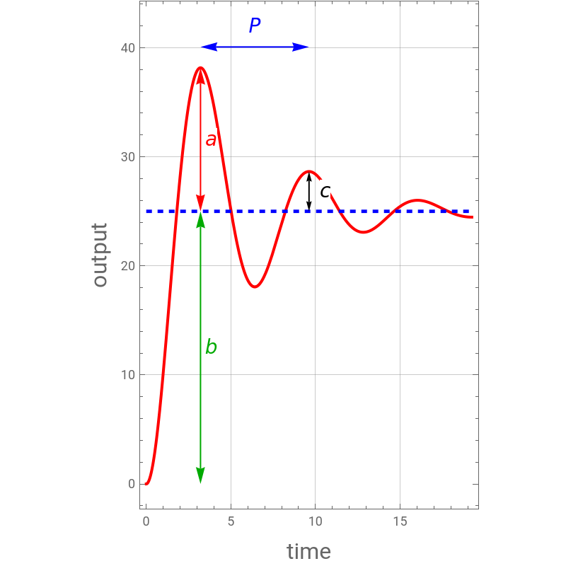
Consider an underdamped second-order process with a transfer function (the ratio of output to input of a system), given by , where is the steady-state gain, is the time constant, and is the damping coefficient (with ). This process is subjected to a step input . Here, we show plots of the response and finds its performance characteristics: overshoot , decay ratio , time to rise , time to first peak , and period of oscillations . These performance characteristics are reported in a Table at the end of the notebook.
G(s)=+2ζτs+1
K
g
2
τ
2
s
K
g
τ
ζ
0<ζ<1
U(t)=
M
s
y(t)=(G(s)U(s))
-1
ℒ
a/b
c/a
t
r
t
p
P
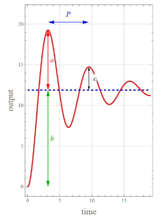
The overshoot is equal to .The decay ratio is equal to .The period of oscillation is .The time to first peak is given by =πτ.The rise time is the solution of and .
a/b=exp-πζ
1-
2
ζ
c/a==exp-2πζ
2
(a/b)
1-
2
ζ
P=2πτ
1-
2
ζ
t
p
1-
2
ζ
t
r
y()=M
t
r
K
g
0<<
t
r
t
p
For illustration purposes, we adopt the following values : Kg = 5; τ = 1; ζ = 0.2; M = 5;
In[]:=
Kg=5;τ=1;ζ=0.2;M=5;
Letusconstruct:y(t)=(G(s)U(s))
-1
ℒ
In[]:=
InvTau=1/τ;ω=Sqrt[InvTau^2-(InvTauζ)^2];
In[]:=
yanal[t_]:=KgM+(-2KgMInvTauζ/ω+KgMInvTauζ/ω)Exp[-ζInvTaut]Sin[ωt]-KgMExp[-ζInvTaut]Cos[ωt];
The time to first peak is given by =πτ.
t
p
1-
2
ζ
In[]:=
tp=Piτ/Sqrt[1-ζ^2];
The period of oscillation is .
P=2πτ
1-
2
ζ
In[]:=
P=2Pi/ω;
In[]:=
sol1=FindRoot[yanal[t]MKg,{t,0,tp}]//Chop;sol2=FindMaximum[yanal[t],{t,tp,tp+0.2}];
In[]:=
sol3=Quiet@FindMaximum[yanal[t],{t,tp+P}];
The overshoot is equal to .The decay ratio is equal to .
a/b=exp-πζ
1-
2
ζ
c/a==exp-2πζ
2
(a/b)
1-
2
ζ
In[]:=
Overshoot=Exp[-Piζ/Sqrt[1-ζ^2]];DecayRatio=Exp[-2Piζ/Sqrt[1-ζ^2]];
In[]:=
p1=Plot[yanal[t],{t,0,3P},FrameTrue,GridLinesAutomatic,AspectRatio1.5,FrameLabel{Style["time",16],Style["output",16]},PlotRangeAll,PlotStyle{Red,Thick},ImageSize400{1,1}];
In[]:=
Show[p1,Graphics[{{Dashed,Thickness[0.01],Blue,Line[{{0,MKg},{3P,MKg}}]},Darker@Green,Arrowheads[{-.05,.05}],Arrow[{{tp,0},{tp,MKg}}],Red,Arrowheads[{-.05,.05}],Arrow[{{tp,MKg},{tp,sol2[[1]]}}],Blue,Arrowheads[{-.05,.05}],Arrow[{{tp,sol2[[1]]1.05},{t/.sol3[[2]],sol2[[1]]1.05}}],Style[Text[Style["P",Italic],{((t/.sol3[[2]])+tp)/2,sol2[[1]]1.1},{0,0}],Blue,14,BackgroundWhite],Style[Text[Style["b",Italic],{tp1.2,MKg/2},{0,0}],Darker@Green,14,BackgroundWhite],Style[Text[Style["a",Italic],{tp1.2,MKg/2+sol2[[1]]/2},{0,0}],Red,14,BackgroundWhite],Style[Text[Style["c",Italic],{(t/.sol3[[2]])1.1,MKg/2+sol3[[1]]/2},{0,0}],Black,14,BackgroundWhite],Black,Arrowheads[{-.03,.03}],Arrow[{{(t/.sol3[[2]]),MKg},{(t/.sol3[[2]]),sol3[[1]]}}]}]]
Out[]=
In[]:=
Text@Style[Grid[{{"property","value"},{Row[{"overshoot ",Style["a",Italic],"/",Style["b",Italic]}],NumberForm[Overshoot,{5,4}]},{Row[{"decay ratio ",Style["c",Italic],"/",Style["a",Italic]}],NumberForm[DecayRatio,{5,4}]},{Row[{"period ",Style["P",Italic]}],NumberForm[P,{5,4}]},{Row[{"rise time ",}],NumberForm[t/.sol1,{5,4}]},{Row[{"time to first peak ",}],NumberForm[tp,{5,4}]}},FrameAll,Background{None,{Lighter[Blend[{Blue,Red}],.8],{Lighter[Blend[{Blue,Darker@Green}],.8],Lighter[Green,.9]}}},ItemSize{9.3,3.3},FrameDarker[Gray,.6],ItemStyle14,Spacings{Automatic,.8}],16]
Style["t",Italic]
"r"
Style["t",Italic]
"p"
Out[]=
property | value |
overshoot a/b | 0.5266 |
decay ratio c/a | 0.2773 |
period P | 6.4127 |
rise time t r | 1.8087 |
time to first peak t p | 3.2064 |
References
References
[1] D. E. Seborg, T. F. Edgar, D. A. Mellichamp, and F. J. Doyle III, Process Dynamics and Control, 4th ed., Hoboken, NJ: John Wiley & Sons, Inc., 2017.
CITE THIS NOTEBOOK
CITE THIS NOTEBOOK
Performance characteristics for step response of an underdamped process
by Housam Binous and Ahmed Bellagi
Wolfram Community, STAFF PICKS, March 21, 2024
https://community.wolfram.com/groups/-/m/t/3145151
by Housam Binous and Ahmed Bellagi
Wolfram Community, STAFF PICKS, March 21, 2024
https://community.wolfram.com/groups/-/m/t/3145151