Breakthrough curves for adsorption
Authors: Housam Binous and Ahmed Bellagi
Breakthrough curves for adsorption
Authors: Housam Binous and Ahmed Bellagi
Authors: Housam Binous and Ahmed Bellagi
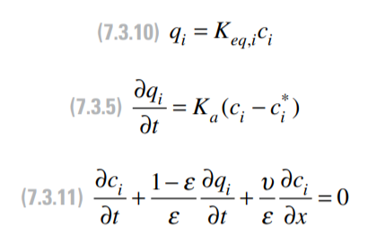
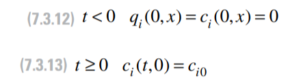
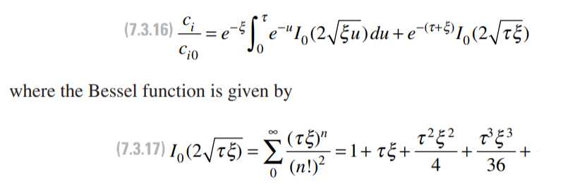
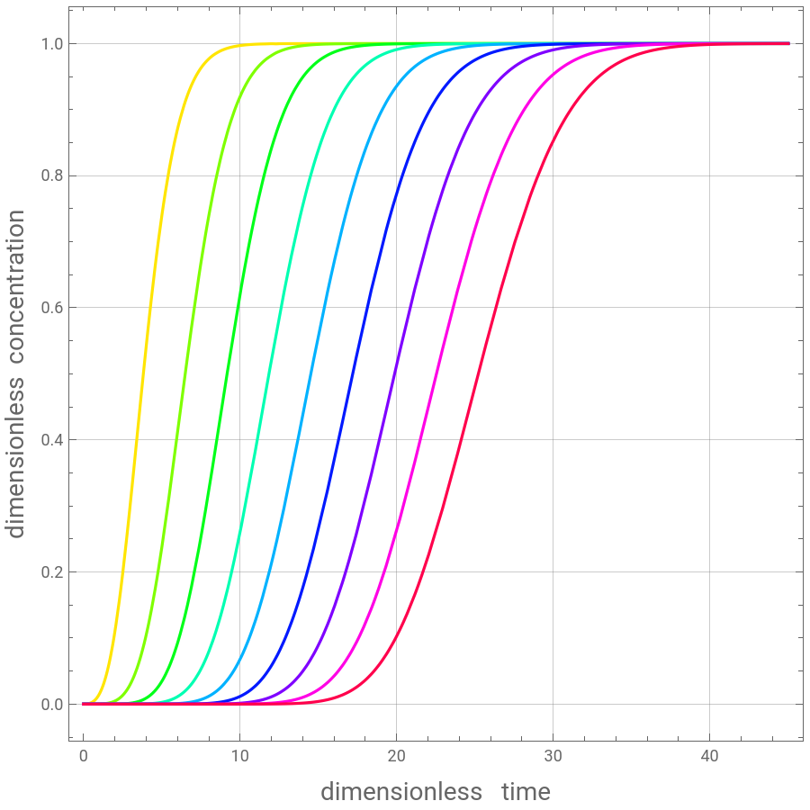
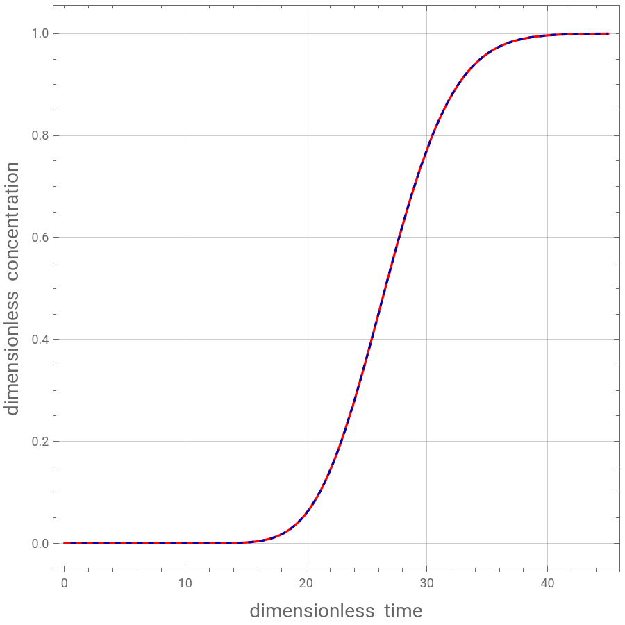
We solve a system of PDEs, describing adsorption assuming linear driving force, negligible dispersion and linear adsorption isotherm, using either NDSolve or Chebyshev Orthogonal Collocation.The resulting breakthrough curves are compared to their counterparts obtained using an analytical expression. We find perfect agreement between the three methods.The governing equations from Harrison et al. (2003): The initial and boundary conditions are:
Acknowledgement: The expression for the analytical solution and governing equations for adsorption assuming linear driving force, negligible dispersion and linear adsorption isotherm were obtained from Harrison et al., Bioseparations Science and Engineering, OUP, 2003.whereReferences:1. Klinkenberg, A. (1954). Heat transfer in cross-flow heat exchangers and packed beds. Ind. Eng. Chem., vol. 46, p. 2285.2. Furnas, C. C. (1930). Heat transfer from a gas stream to a bed of broken solids. Trans. AIChE, vol. 24, p. 142.
Numerical solution for the breakthrough curves. Results are identical to Harrison at al.
In[]:=
Ka=105;Keq=40;v=20;ϵ=0.34;
In[]:=
sol=NDSolve[{D[qi[t,x],{t,1}]Ka(ci[t,x]-1/Keqqi[t,x]),D[ci[t,x],{t,1}]+(1-ϵ)/ϵD[qi[t,x],{t,1}]+v/ϵD[ci[t,x],{x,1}]0,qi[0,x]0,ci[0,x]Exp[-10^20x],ci[t,0]1},{ci[t,x],qi[t,x]},{x,0,20},{t,0,45},Method{"MethodOfLines","SpatialDiscretization"{"TensorProductGrid","MinPoints"100}},PrecisionGoal10]
Out[]=
ci[t,x]InterpolatingFunction[t,x],qi[t,x]InterpolatingFunction[t,x]


In[]:=
p1=Show[Table[Plot[Evaluate[ci[t,x]/.sol/.xξ],{t,0,45},PlotRangeAll,PlotLegendsTable[Style[,Black],{i,3,20,2}],PlotStyleHue[ξ/20],AspectRatio1,ImageSize450{1,1},GridLinesAutomatic,FrameTrue,FrameLabel{Style["dimensionless time",14],Style["dimensionless concentration",14]}],{ξ,3,20,2}]]
c
ξ
Out[]=


Analytical expression for the breakthrough curves (for details about derivation of the analytical solution see Refs. 1 and 2)
In[]:=
analyt[τ_?NumericQ,ξ_?NumericQ]:=Exp[-ξ]NIntegrateExp[-u]BesselI0,2.
ξu
,{u,0,τ}+Exp[-(τ+ξ)]BesselI0,2.ξτ
In[]:=
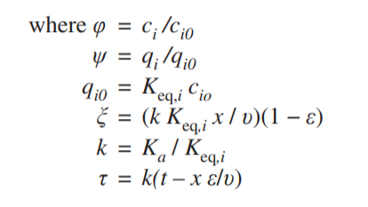
solξ=Solve[(Kax/v(1-ϵ)/.x20)ξ,ξ]
Out[]=
{{ξ69.3}}
In[]:=
solτ=Solve[(τKa/Keq(t-xϵ/v)/.x20),τ]
Out[]=
{{τ2.625(-0.34+t)}}
In[]:=
plotanalyt=Quiet@Plot[Evaluate[analyt[τ,ξ]/.solξ/.solτ],{t,0.5,45},PlotStyle{Darker@Blue,Dashed},PlotRangeAll,AspectRatio1,GridLinesAutomatic,FrameTrue,FrameLabel{Style["dimensionless time",14],Style["dimensionless concentration",14]}]
Out[]=
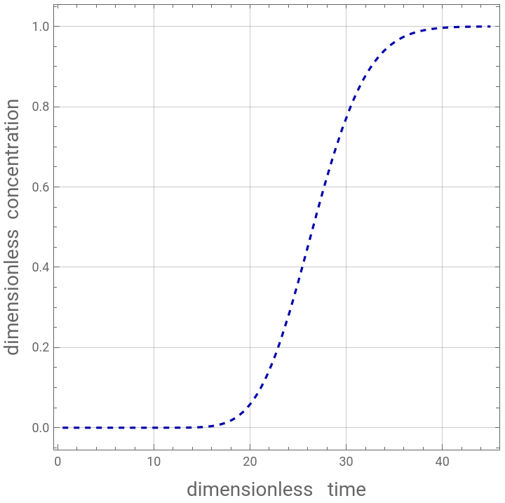
Conclusion: Numerical and analytical breakthrough curves and identical @ x=20
In[]:=
Show[Show[Table[Plot[Evaluate[ci[t,x]/.sol/.xξ],{t,0,45},PlotRangeAll,PlotLegendsTable[Style[,Black],{i,3,20,2}],PlotStyleHue[ξ/20],AspectRatio1,GridLinesAutomatic,FrameTrue,FrameLabel{Style["dimensionless time",14],Style["dimensionless concentration",14]}],{ξ,20,20,2}]],plotanalyt,ImageSize450{1,1}]
c
ξ
Out[]=

Constructing the derivative matrices for Chebyshev orthogonal collocation
Constructing the derivative matrices for Chebyshev orthogonal collocation
Comparison of solution using Chebyshev orthogonal collocation (colored curves) and its counterpart obtained using NDSolve (dashed gray curves)
Comparison of solution using Chebyshev orthogonal collocation (colored curves) and its counterpart obtained using NDSolve (dashed gray curves)