This computational essay presents a comprehensive exploration of super-oscillatory behavior across several two-dimensional wave systems. We begin by analyzing random isotropic superpositions of monochromatic plane waves, numerically verifying the theoretical probability of super-oscillations in D dimensions and demonstrating how phase vortices naturally emerge at nodal line intersections. Then we move on to show the relation of the quantum potential and super-oscillation regions applied to 2D band-limited functions and Aharonov-Bohm scattering waves. Finally, we investigate the time evolution of exponential power states, explicitly computing their momentum spectra, off-center vortex locations, and the dynamics of their super-oscillatory structures.
Monochromatic 2D waves
Monochromatic 2D waves
For two dimensional case of monochromatic waves we consider an isotropic superposition of plane waves, such that are random complex numbers and the directions / are uniformly distributed constant):
a
n
k
n
k
0
(
k
0

(
1
)Setting the value =2π and the number of waves:
k
0
In[]:=
k0=2Pi;Nwaves=10;SeedRandom[44];
Generate and :
a
n
k
n
In[]:=
kn=FromPolarCoordinates@Thread[{k0,RandomReal[{-π,π},Nwaves]}];an=RandomComplex[{-1-I,1+I},Nwaves];
Calculate the overall function ψ( function:
x,y)
In[]:=
psi=Total[anExp[(kn.{x,y})]];
Local wavenumber vector and norm:
In[]:=
kLocalVec=Im;kLocal=Norm[kLocalVec];
Grad[psi,{x,y}]
psi
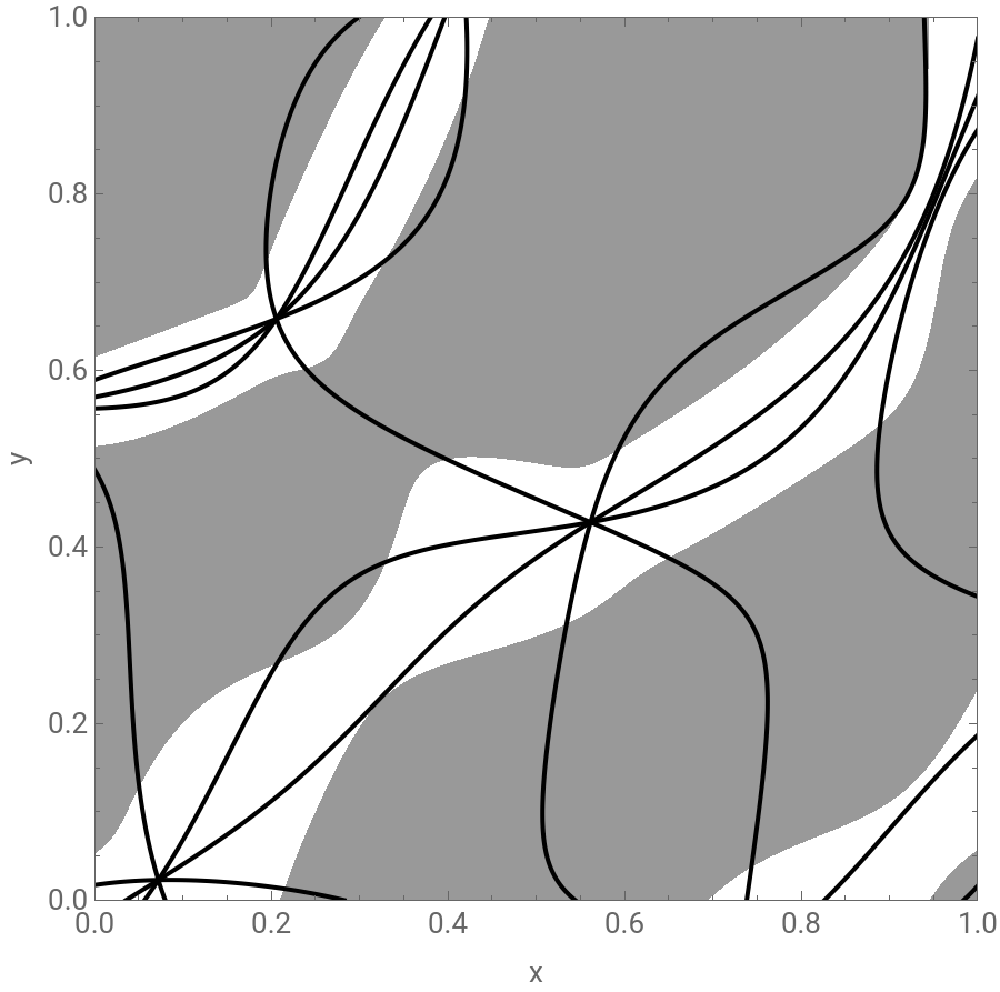
Show super-oscillations regions (transparent regions) where ||:
k
local
>
k
0
In[]:=
shading=ContourPlot[kLocal,{x,0,1},{y,0,1},Contours->{k0},ContourShading->{GrayLevel[0.6],Transparent},ContourStyle->None,PlotPoints->80];
Generate a plot of contours of the phase in intervals of π/4:
In[]:=
phaseContours=ContourPlot[{Re[psi]==0,Im[psi]==0,-Re[psi]+Im[psi]==0,Re[psi]+Im[psi]==0},{x,0,1},{y,0,1},ContourStyle->Black,PlotPoints->120];
Visualize the combined plot:
In[]:=
Show[shading,phaseContours,Frame->True,AspectRatio->1,PlotRangePadding->None,LabelStyle->13,FrameLabel->{"x","y"},ImageSize->450]
Out[]=
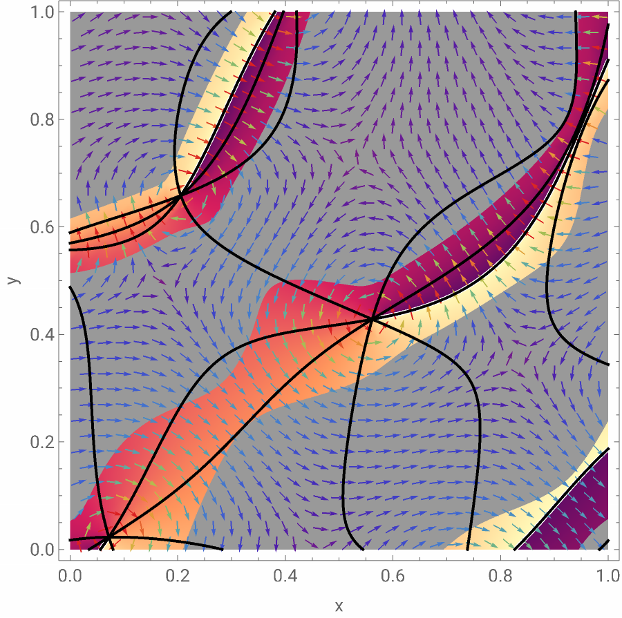
Phase vortices appear precisely where the black lines in the previous plot intersect, we can visualize this accompanied by the vector plot of and the density plot of the phase:
k
Local
In[]:=
g1=VectorPlot[kLocalVec,{x,0,1},{y,0,1},StreamColorFunction->None,StreamStyle->Black,PlotLegends->BarLegend[Automatic,LegendLabel->"||"],VectorColorFunction->"Rainbow",VectorPoints->30];g2=DensityPlot[Arg[psi],{x,0,1},{y,0,1},FrameLabel->{"x","y"},LabelStyle->13];Show[g2,shading,g1,phaseContours,ImageSize->450]
k
Local
Out[]=

Calculate the singularities points:
In[]:=
singularities=Quiet@NSolve[{Re[psi]==0,Im[psi]==0,0<=x<=1,0<=y<=1},{x,y}]
Out[]=
{{x0.0721117,y0.0228474},{x0.205748,y0.658355},{x0.561546,y0.428115}}
Fly-byes of the wavefunction at the values of the phase singularities:
y
In[]:=
flybyes=psi/.List/@singularities[[All,2]];Plot[Evaluate[Log@Abs@Re[flybyes]],{x,0,1},PlotRange->All,AxesLabel->{"x"},LabelStyle->12]
Out[]=
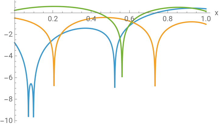
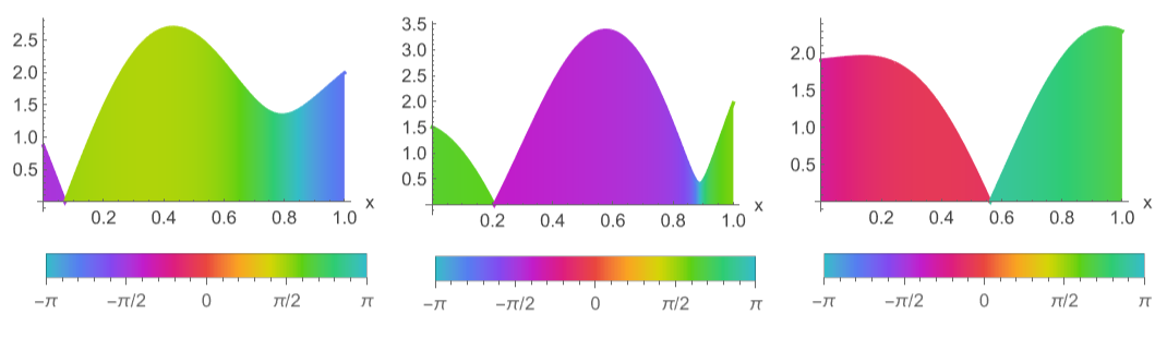
The plot of Log|Re(ψ)| did not tell us much, but we can recognize the super-oscillations in zones with a rapid change of phase:
In[]:=
GraphicsRow[AbsArgPlot[#,{x,0,1},PlotLegends->Automatic,Filling->Bottom,ImageSize->200,AxesLabel->{"x"}]&/@flybyes,ImageMargins->0]
Out[]=
Fourier components of the first flyby:
In[]:=
FourierTransform[flybyes[[1]],x,kx]
Out[]=
(-1.72636-0.960571)DiracDelta[(4.50315+0.)-kx]+(0.553312-2.13687)DiracDelta[(5.00737+0.)-kx]-(0.313963-0.0922222)DiracDelta[(5.5219+0.)-kx]-(0.45229-1.42494)DiracDelta[(5.88034+0.)-kx]+(0.555279+0.642321)DiracDelta[(6.0795+0.)-kx]-(1.72516+0.825511)DiracDelta[(6.22343+0.)-kx]+(1.63266+1.35383)DiracDelta[(3.04152+0.)+kx]+(1.93763+0.0230841)DiracDelta[(4.54758+0.)+kx]-(0.17993+2.42557)DiracDelta[(4.87735+0.)+kx]-(0.12568-0.648339)DiracDelta[(6.26395+0.)+kx]
Of course all the wave-vector components of the flyby should have magnitude than :
less
k
0
In[]:=
AllTrue[Flatten@Cases[%,DiracDelta[a_]:>SolveValues[a==0,kx],∞],Abs[#]<k0&]
Out[]=
True
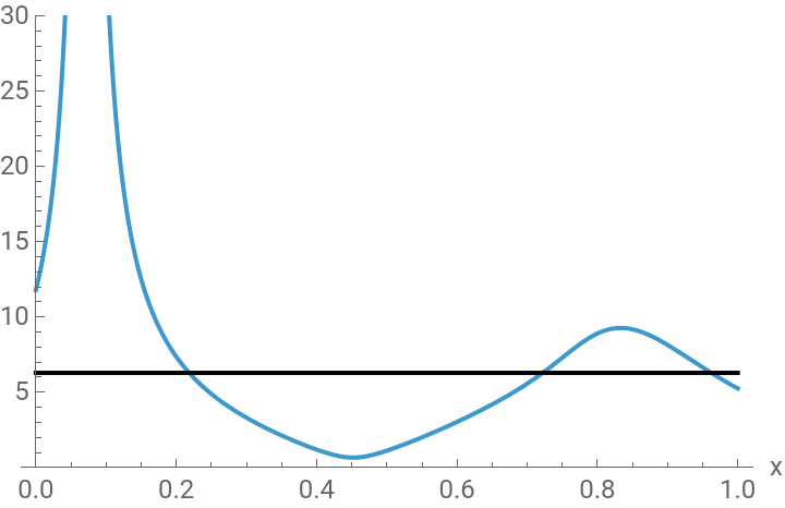
Compare the local wave-vector of the first flyby to :
k
0
In[]:=
Plot[{kLocal/.singularities[[1,2]],k0},{x,0,1},PlotRange->{0,30},AxesLabel->{"x"},PlotStyle->{Automatic,Black},LabelStyle->12,PlotLegends->{"",""}]
k
Local
k
0
Out[]=


For the two dimensional case we get:
The mean of those values should be close to 1/3:
Super-oscillations and the quantum potential
Super-oscillations and the quantum potential
Madelung-Bohm formalism polar representation:
Replacing in Eq.(4) we can get the following two equations:
Such that we can define the quantum potential, quantum kinetic momentum and classical kinetic momentum as:
Berry 2D function
Berry 2D function
It is possible to extend the Fourier components to construct a two dimensional function that is a band-limited superposition of non-evanescent plane waves:
Calculate the local wave-vector:
Contour plot of the phase of the function and magnitude of the local wave-vector:
Calculate the number of singularities in the rectangle from -2π to 2π :
Zoom in one the phase vortex:
A zoom-in of the region near the origin reveals the presence of two phase vortices. The phase of the flybys, corresponding to the dashed blue lines in the left plot, exhibits a maximum change upon crossing these vortices:
Visualize the super-oscillatory zone:
It has 16 phase vortices in the square region from - 2π to 2π :
All the Fourier components have wave-vector magnitude of 1:
Now define a super\bposition with different parameters:
Phase and magnitude behavior:
Aharonov-Bohm(AB) waves
Aharonov-Bohm(AB) waves
where Φ represents the flux of the magnetic field concentrated in a line
Differential operator of the given equation:
Check the elementary function is a solution:
Quoting Berry: “This is a subtle matter, involving mathematical technicalities. But since the wave outside the flux line moves in a plane free of electric and magnetic fields it is a reasonable extension of terminology describe the fast variations of these waves as super-oscillations”
The zeros of the quantum potential that can delimit the regions of fast oscillations can also be expressed as a condition for the kinetic wave-vector:
Construct the AB wave, instead of the infinite sum we use a truncated approximation:
Kinetic and local wave-vector:
We consider a free quantum particle in 2-dimension, initially prepared in a “radially symmetric” state
Exponential power state
Exponential power state
Initial wave function (without normalization):
Evolved wave function (free evolution), the time-evolved wave function is derived using the free-space Green’s function:
Defining it in Cartesian coordinates:
Probability density in momentum space:
Initial state
Initial state
Check normalization condition:
Linear superposition for potential super-oscillations
Linear superposition for potential super-oscillations
Define two wavefunction with close radial parameter that have complex values:
Check the normalization:
We can solve for that point numerically:
In Cartesian coordinates:
Expressing the variables with the parameters that were used before:
Normalization constants:
Solving the magnitude equation:
Set the phase difference to π (or - π):
We see there is a change of behavior of the phase at the point that was calculated:
Express the required functions in Cartesian coordinates:
In the zoom-in we can visualize clearly the other phase vortex behavior:
Plot the function:
Check normalization:
We there is a small localized fast-oscillation zone around the off center vortex:
Time evolution (μ = n +1)
Time evolution (μ = n +1)
Using that simplified function it is possible to derive the following results
Total phase:
Local wave-vector:
The only phase vortex is at the origin:
Express the local wave-vector field in Cartesian coordinates:
But there can be a change of the vortex geometric structure, in this case circular pattern disappearance:
Using α = 0.2 + 0.4 , n = 5 there is circular pattern appearance:
Evolution μ = n - 1
Evolution μ = n - 1
Simplified wave function:
Total phase:
Local momentum:
Although radial spreading is an expected consequence of time evolution, this suggests that for superimposed states, there should be a critical time window optimal for generating rapid off-center “super-oscillations”
Conclusions
Conclusions
◼
Super-oscillatory region where the local wave-vector exceeds the maximum plane-wave Fourier components, naturally emerge in complex wave superpositions and are intrinsically linked to the presence and geometry of phase singularities
◼
The zeros of the quantum potential serve as geometrical delimiters of fast-oscillation regions
◼
The analysis done for time evolution of radial symmetric functions can still be improved, a critical question is to ask what happens to the time evolution of a superposition and formalize if there exists a favorable super-oscillatory time window
References
References
◼
[1] Berry, M. V., & Dennis, M. R. (2009). Natural super-oscillations in monochromatic waves in D dimensions. Journal of Physics A: Mathematical and Theoretical, 42(2), 022003.
◼
[2] Gradshteyn, I. S., & Ryzhik, I. M. (2014). Table of integrals, series, and products. Academic press.
◼
[3] Berry, M. V. (2020). Super-oscillations and the quantum potential. European Journal of Physics, 42(1), 015401.
CITE THIS NOTEBOOK
CITE THIS NOTEBOOK
Superoscillations Part 2: Phase vortices, quantum potential and free evolution of wave packets
by Bruno Tenorio
Wolfram Community, STAFF PICKS, June 1, 2026
https://community.wolfram.com/groups/-/m/t/3725403
by Bruno Tenorio
Wolfram Community, STAFF PICKS, June 1, 2026
https://community.wolfram.com/groups/-/m/t/3725403