Quantum Mechanics
Quantum Mechanics
Normalization and Probabilities
Relative Statistics
Relative Statistics
Expectation value ( μ ): 〈 〉 = ∫ ψ dxStandard Deviation ( σ ): =
k
x
*
ψ
k
x
σ
x
〈〉-〈x
2
x
2
〉
Patterns
Patterns
In[]:=
(*complexconjugate*)
In[]:=
*
φ_
(*innerprodutwithoptionaloperatorandbounds*)
In[]:=
InnerProduct[〈φ_,k_:1,ψ_〉,lower_:-Infinity,upper_:Infinity]:=Integrate[kψ,{x,lower,upper}]
*
φ
In[]:=
(*momentumoperator*)
In[]:=
p
k
ℏ
I
In[]:=
p
1
ℏ
∂
{x,1}
In[]:=
p
Out[]=
-ℏ[x]
′
ψ
Examples
Examples
Time Independent Wave Function
Time Independent Wave Function
0 x < 0 ψ( x ) = { A 0 ≤ x ≤ c 0 c < x
2
x
2
(x-c)
Determine normalization constant “A”
Evaluate 〈 x 〉, 〈 〉 and
2
x
σ
x
Evaluate 〈 p 〉, 〈 〉 and
2
p
σ
p
Compute ,
σ
x
σ
p
In[]:=
$Line=0;
In[]:=
(*definewavefunction*)
In[]:=
ψ[x_/;x<0]:=0ψ[x_]:=A
2
x
2
(x-c)
In[]:=
DownValues@ψ
Out[]=
{HoldPattern[ψ[x_/;x<0]]0,HoldPattern[ψ[x_]]A}
2
x
2
(x-c)
In[]:=
(*solvefornormalizationconstantandupdateDownValue*)
In[]:=
Solve[InnerProduct[〈ψ[x],ψ[x]〉,0,c]1,A][[2,1]]
Out[]=
A
3
70
9/2
c
In[]:=
ψ[x_]=ψ[x]/.%;(*replaceAwiththepreviouslycomputedoutput*)
In[]:=
DownValues@ψ
Out[]=
HoldPattern[ψ[x_/;x<0]]0,HoldPattern[ψ[x_]]
3
70
2
x
2
(-c+x)
9/2
c
In[]:=
(*showthatthecorrectconstanthasbeendetermined*)
In[]:=
InnerProduct[〈ψ[x],ψ[x]〉,0,c]==1
In[]:=
True(*correctnormalizationconstantfound*)
In[]:=
(*Evaluating〈x〉,〈〉,*)
2
x
σ
x
In[]:=
#,#2,})
#2-
&@@(InnerProduct[〈ψ[x],#,ψ[x]〉,0,c]&/@{x,2
#
2
x
Out[]=
,,
c
2
3
2
c
11
2
c
2
11
In[]:=
(*Evaluating〈p〉,〈〉,*)
2
p
σ
p
In[]:=
#,#2,[#,x]@ψ[x],0,c&/@{1,2}
#2-
&@@InnerProductψ[x],2
#
p
Out[]=
0,,2
12
2
ℏ
2
c
3
2
ℏ
2
c
In[]:=
(*>ℏ/2*)
σ
x
σ
p
In[]:=
Out[10][[3]]Out[14][[3]]
Out[]=
3
11
2
c
2
ℏ
2
c
In[]:=
unc=%Assuming[c>0&&ℏ>0,Refine@(unc>ℏ/2)]
Out[]=
3
11
2
c
2
ℏ
2
c
Out[]=
True
Time dependent Wave Function
Time dependent Wave Function
Determine the normalization constant ‘n’
Is the probability of finding the particle in the interval (L, ∞) and t = 0 different from the probability at t = 10?
What is the probability of finding the particle in the interval ( 〈 x 〉 - , 〈 x 〉 + )?
σ
x
σ
x
(*SetGlobalassumption*)
In[]:=
$Assumptions=L∈Reals&&L>0;
(*Definingthewavefunction*)
In[]:=
Ψ[x_,t_]:=nExp--t
Abs@x
L
eneI
ℏ
In[]:=
DownValues@Ψ
Out[]=
HoldPattern[Ψ[x_,t_]]nExp--
Abs[x]
L
(ene)t
ℏ
(*Normalizationcoefficient*)
Solve[InnerProduct[〈Ψ[x,t],Ψ[x,t]〉]1,n][[2,1]]Ψ[x_,t_]=Ψ[x,t]/.%;(*findpattern{Ψ[x,t]}replace{/.}'n'withthepreviousoutput{%}*)
Out[]=
n
enet
ℏ
L
In[]:=
DownValues@Ψ
In[]:=
HoldPattern[Ψ[x_,t_]]
-
Abs[x]
L
L
(*innerproductoverthespecifiedinterval*)
In[]:=
{#,N@#}&@InnerProduct[〈Ψ[x,t],Ψ[x,t]〉,L,Infinity](*{#,N@#}symbolic_value,numeric_value;&endoffunction,@affix*)
Out[]=
,0.0676676
1
2
2
(*<x>,<>,*)
2
x
σ
x
In[]:=
{lower,upper}={#-#3,#+#3}&@@#,#2,})
#2-
&@@(InnerProduct[〈Ψ[x,t],#,Ψ[x,t]〉]&/@{x,2
#
2
x
Out[]=
-,
2
L
2
2
L
2
In[]:=
{#,N@#}&@InnerProduct[〈Ψ[x,t],Ψ[x,t]〉,lower,upper]
Out[]=
(-1+),0.756883
-
2
2
(*Potting*)
In[]:=
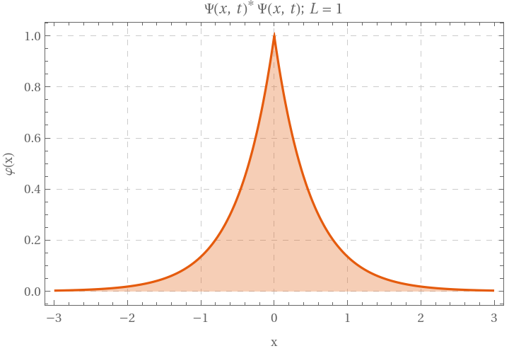
Plot[Evaluate[Ψ[x,t]/.L1.],{x,-3.,3.},FillingAxis,GridLinesAutomatic,GridLinesAutomatic,GridLinesStyleDirective[Dashed,GrayLevel[0.8]],FrameLabel{"x","φ(x)"},PlotLabelHoldForm[Ψ[x,t];L=1],PlotTheme"Scientific"]
*
Ψ[x,t]
*
Ψ[x,t]
Out[]=