Problem 11-60 reproduced from Ref. 1
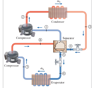
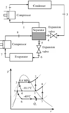
A two-stage compression refrigeration system with an adiabatic liquid-vapor separation unit as shown in Fig. P11–60 uses refrigerant-134a as the working fluid. The system operates the evaporator at −40°C, the condenser at 800 kPa, and the separator at 10.1°C. This system is to serve a 30-kW cooling load.
Determine the mass flow rate through each of the two compressors, the power used by the compressors, and the system’s COP. The refrigerant is saturated liquid at the inlet of each expansion valve and saturated vapor at the inlet of each compressor, and the compressors are isentropic.
Reference:
[1] Çengel, Yunus A., Boles, Michael A., Kanoğlu, Mehmet, Thermodynamics: An Engineering Approach, Ninth Edition, NY: McGraw-Hill, 2019.
R134A saturation properties - temperature increment Temperature (C) Pressure (bar) Enthalpy (kJ/kg) Entropy (J/g*K) Enthalpy (kJ/kg) Entropy (J/g*K)
datasat=;
In[]:=
tblhl=Table[{datasat[[i]][[2]],datasat[[i]][[3]]},{i,1,Length[datasat]}];tblsl=Table[{datasat[[i]][[2]],datasat[[i]][[4]]},{i,1,Length[datasat]}];fhl=Interpolation[tblhl,InterpolationOrder1];fsl=Interpolation[tblsl,InterpolationOrder1];tblhv=Table[{datasat[[i]][[2]],datasat[[i]][[5]]},{i,1,Length[datasat]}];tblsv=Table[{datasat[[i]][[2]],datasat[[i]][[6]]},{i,1,Length[datasat]}];fhv=Interpolation[tblhv];fsv=Interpolation[tblsv];tbltp=Table[{datasat[[i]][[1]],datasat[[i]][[2]]},{i,1,Length[datasat]}];ftp=Interpolation[tbltp];
In[]:=
P5=P1;P1=ftp[-10.1]
Out[]=
1.99812
In[]:=
H1=fhv[P1]
Out[]=
244.46
In[]:=
H5=fhl[P5]
Out[]=
38.4193
In[]:=
P7=ftp[-40.]
Out[]=
0.512092
In[]:=
H6=H5
Out[]=
38.4193
In[]:=
H7=fhv[P7]
Out[]=
225.863
In[]:=
H4=H3;
In[]:=
P3=8;
In[]:=
H3=fhl[P3]
Out[]=
95.5004
In[]:=
S7=fsv[P7]
Out[]=
0.968727
In[]:=
S8=S7
Out[]=
0.968727
In[]:=
P8=P1
Out[]=
1.99812
R134A isobaric properties - pressure = 1.998 bar
Temperature (C) Pressure (bar) Enthalpy (kJ/kg) Entropy (J/g*K) Phase
Temperature (C) Pressure (bar) Enthalpy (kJ/kg) Entropy (J/g*K) Phase
dataisobaric=;
In[]:=
pos=Position[dataisobaric,-10.102]
Out[]=
{{198,1},{199,1}}
In[]:=
tblhsv=Table[{dataisobaric[[i]][[1]],dataisobaric[[i]][[3]]},{i,199,Length[dataisobaric]}];tblssv=Table[{dataisobaric[[i]][[1]],dataisobaric[[i]][[4]]},{i,199,Length[dataisobaric]}];tblshsv=Table[{dataisobaric[[i]][[4]],dataisobaric[[i]][[3]]},{i,199,Length[dataisobaric]}];
In[]:=
fshsv=Interpolation[tblshsv];
In[]:=
tblhl1=Table[{datasat[[i]][[3]],datasat[[i]][[2]]},{i,1,Length[datasat]}];tblsl1=Table[{datasat[[i]][[4]],datasat[[i]][[1]]},{i,1,Length[datasat]}];
In[]:=
tblhv1=Table[{datasat[[i]][[5]],datasat[[i]][[2]]},{i,1,Length[datasat]}];tblsv1=Table[{datasat[[i]][[6]],datasat[[i]][[1]]},{i,1,Length[datasat]}];
In[]:=
fhsv=Interpolation[tblhsv];
In[]:=
fssv=Interpolation[tblssv];
In[]:=
H8=fshsv[S8]
Out[]=
252.742
R134A isobaric properties - pressure = 8.0 bar
Temperature (C) Pressure (bar) Enthalpy (kJ/kg) Entropy (J/g*K) Phase
Temperature (C) Pressure (bar) Enthalpy (kJ/kg) Entropy (J/g*K) Phase
dataisobaric2=;
In[]:=
pos=Position[dataisobaric2,31.328]
Out[]=
{{284,1},{285,1}}
In[]:=
tblhsv=Table[{dataisobaric2[[i]][[1]],dataisobaric2[[i]][[3]]},{i,285,Length[dataisobaric2]}];tblssv=Table[{dataisobaric2[[i]][[1]],dataisobaric2[[i]][[4]]},{i,285,Length[dataisobaric2]}];tblshsv=Table[{dataisobaric2[[i]][[4]],dataisobaric2[[i]][[3]]},{i,285,Length[dataisobaric2]}];
In[]:=
fshsv2=Interpolation[tblshsv];
In[]:=
fhsv2=Interpolation[tblhsv];
In[]:=
fssv2=Interpolation[tblssv];
In[]:=
S1=fsv[P1]
Out[]=
0.937809
In[]:=
S2=S1
Out[]=
0.937809
In[]:=
H2=fshsv2[S2]
Out[]=
273.27
In[]:=
sol=NSolve[{QDOTL==mdot6(H7-H6),mdot6(H8-H5)==mdot2(H1-H4),WDOTIN==mdot6(H8-H7)+mdot2(H2-H1),QDOTL==30},{QDOTL,mdot2,mdot6,WDOTIN}]
Out[]=
{{QDOTL30.,mdot20.230277,mdot60.160048,WDOTIN10.9362}}
In[]:=
COP=First[QDOTL/WDOTIN/.sol]
Out[]=
2.74319