ABSTRACT (original article): We look at curvatures that are supported on k-dimensional parts of a simplicial complex G. These curvature all satisfy the Gauss-Bonnet theorem, provided that the k-dimensional simplices cover . Each of these curvatures can be written as an expectation of Poincare-Hopf indices. Linear or non-linear wave dynamics with discrete or continuous time allow to deform these curvatures while keeping the Gauss-Bonnet property. CITATION (original article): Oliver Knill (2024), Gauss-Bonnet for Form Curvatures, arXiv:2409.01425. https://doi.org/10.48550/arXiv.2409.01425
G
Here is the Mathematica code included in the https://arxiv.org/abs/2409.01425 with abstract “We look at curvatures that are supported on k-dimensional parts of a simplicial complex G. These curvature all satisfy the Gauss-Bonnet theorem, provided that the k-dimensional simplices cover G. Each of these curvatures can be written as an expectation of Poincare-Hopf indices. Linear or non-linear wave dynamics with discrete or continuous time allow to deform these curvatures while keeping the Gauss-Bonnet property”. The motivation for this paper had been to explore a wider variety of curvatures satisfying Gauss-Bonnet. Originally, we wanted to have a good curvature candidate for sectional curvature. The following Mathematica lines should be pretty self-explanatory. We tried to be short as brevity can also be a clarity enhancer. Mathematica allows to write short code. It can handle arbitrary graphs or simplicial complexes. See the linked paper for more details.
In[]:=
Generate[A_]:=If[A=={},{},Sort[Delete[Union[Sort[Flatten[Map[Subsets,A],1]]],1]]];Cl[G_]:=Union[Sort[Map[Sort,G]]];L=Length;sig[x_]:=Signature[x];Bin=Binomial;Rk=MatrixRank;Whitney[s_]:=Cl[Generate[FindClique[s,Infinity,All]]];nu[A_]:=If[A=={},0,L[A]-Rk[A]];F[G_]:=Module[{l=Map[L,G]},If[G=={},{},Table[Sum[If[l[[j]]==k,1,0],{j,L[l]}],{k,Max[l]}]]];sig[x_,y_]:=If[SubsetQ[x,y]&&(L[x]==L[y]+1),sig[Prepend[y,Complement[x,y][[1]]]]*sig[x],0];Dirac[G_]:=Module[{f=F[G],b,d,n=L[G]},b=Prepend[Table[Sum[f[[l]],{l,k}],{k,L[f]}],0];d=Table[sig[G[[i]],G[[j]]],{i,n},{j,n}];{d+Transpose[d],b}];Hodge[G_]:=Module[{Q,b,H},{Q,b}=Dirac[G];H=Q.Q;Table[Table[H[[b[[k]]+i,b[[k]]+j]],{i,b[[k+1]]-b[[k]]},{j,b[[k+1]]-b[[k]]}],{k,L[b]-1}]];omega[x_]:=(-1)^(L[x]-1);Betti[s_]:=Module[{G},If[GraphQ[s],G=Whitney[s],G=s];Map[nu,Hodge[G]]];Fvector[A_]:=Delete[BinCounts[Map[L,A]],1];Euler[A_]:=Sum[omega[A[[k]]],{k,L[A]}];UnitSphere[s_,v_]:=VertexDelete[NeighborhoodGraph[s,v],v];OpenStar[G_,x_]:=Select[G,SubsetQ[#,x]&];deg[G_,x_,k_]:=F[OpenStar[G,x]][[k+1]];Curvatures[s_,k_,t_]:=Module[{G,A,B,Q},If[GraphQ[s],G=Whitney[s],G=s];If[t>0,Q=First[Dirac[G]];U=Re[MatrixExp[t*I*Q]],U=IdentityMatrix[Length[G]]];A=Select[G,(L[#]==k+1)&];If[L[Union[Flatten[A]]]<L[Union[Flatten[G]]],Print["No cover"]];Table[y=A[[l]];Sum[x=G[[i]];omega[x]*U[[i,i]]*If[SubsetQ[y,x],1/deg[G,x,k],If[SubsetQ[x,y],1/Bin[L[x],k+1],0]],{i,L[G]}],{l,L[A]}]];Curvatures[s_,k_]:=Curvatures[s,k,0];
A 4-sphere example
A 4-sphere example
In[]:=
foursphere=CompleteGraph[{2,2,2,2,2}];G=Whitney[foursphere];Betti[G](*Bettinumbers*)Euler[G](*EulerChareacteristic*)
Out[]=
{1,0,0,0,1}
Out[]=
2
Curvatures on vertices = 0 - simplices
In[]:=
C0=Curvatures[G,0]
Out[]=
,,,,,,,,,
1
5
1
5
1
5
1
5
1
5
1
5
1
5
1
5
1
5
1
5
Curvatures on edges = 1 - simplices
In[]:=
C1=Curvatures[G,1]
Out[]=
,,,,,,,,,,,,,,,,,,,,,,,,,,,,,,,,,,,,,,,
1
20
1
20
1
20
1
20
1
20
1
20
1
20
1
20
1
20
1
20
1
20
1
20
1
20
1
20
1
20
1
20
1
20
1
20
1
20
1
20
1
20
1
20
1
20
1
20
1
20
1
20
1
20
1
20
1
20
1
20
1
20
1
20
1
20
1
20
1
20
1
20
1
20
1
20
1
20
1
20
Curvatures on triangles = 2 - simplices
In[]:=
C2=Curvatures[G,2]
Curvatures on tetraedra = 3 - simplices
In[]:=
C3=Curvatures[G,3]
Curvatures on 4 - simplices
In[]:=
C4=Curvatures[G,4]
In[]:=
{Total[C0],Total[C1],Total[C2],Total[C3],Total[C4]}
Out[]=
{2,2,2,2,2}
A random graph
A random graph
In the following example, we compute the edge curvature of a random graph with 20 vertices and 50 edges . As long as there are no isolated vertices, the total edge curvature is the Euler characteristic
In[]:=
s=RandomGraph[{20,50}];{Total[Curvatures[s,1]],Euler[Whitney[s]]}
Out[]=
{-10,-10}
Lets see how the curvatures move if we apply the wave dynamics.
In[]:=
Manipulate[ListPlot[Sort[Curvatures[s,1,t]],PlotRange->{-1,1}],{t,0,3},SaveDefinitions->True]
Out[]=


A homology sphere
A homology sphere
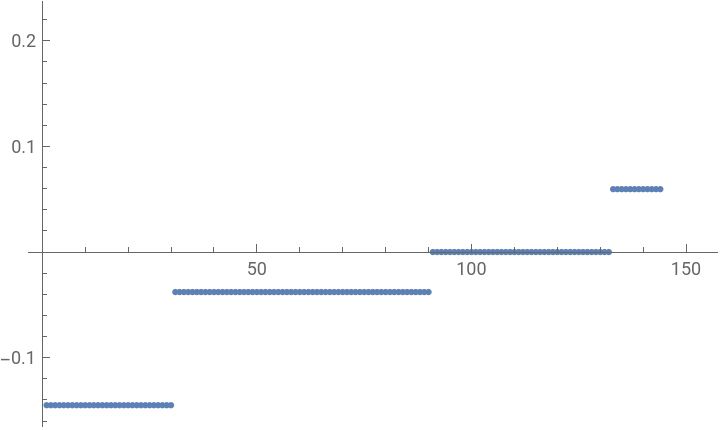
The Poincare-homology sphere is a 3-manifold and so has zero Euler characteristic. We plot the edge curvatures
In[]:=
G=HomologySphere=Generate;C1=Curvatures[G,1];{Total[C1],Euler[G]}ListPlot[Sort[C1]]
Out[]=
{0,0}
Out[]=
CP2
CP2
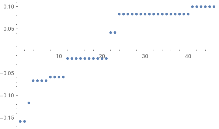
The complex projective space is an example of a 4 manifold which has Euler characteristic 1. The 2,3,4 dimensional curvatures are constant but the 1 dimensional curvature is interesting.
In[]:=
G=CP2=Generate;C1=Curvatures[G,1];{Total[C1],Euler[G]}ListPlot[Sort[C1]]
Out[]=
{1,1}
Out[]=
Wave Evolution
Wave Evolution
In[]:=
Triangles[s_]:=Select[Whitney[s],(Length[#]==3)&];ToGraph[G_]:=UndirectedGraph[n=L[G];Graph[Range[n],Select[Flatten[Table[k->l,{k,n},{l,k+1,n}],1],(SubsetQ[G[[#[[2]]]],G[[#[[1]]]]])&]]];GraphPos[s_]:=Module[{},If[Length[VertexList[s]]<1000,GraphPlot3D[s][[1,1]],GraphPlot3D[s][[1,2,2,1]]]];CurvatureGemPlot[s_,tt_,opts___]:=Module[{p,v,e,t,G=s,F,PS,A1,A2,A3,A,flag=True},p=GraphPos[G];v=VertexList[G];e=EdgeList[G];t=Triangles[G];e=Sort[Table[Sort[{e[[k,1]],e[[k,2]]}],{k,Length[e]}]];rho=Max[Table[Norm[p[[k]]-p[[1]]],{k,Length[p]}]]/40;If[L[t]==0,flag=False];FF=Table[v[[k]]->p[[k]],{k,Length[v]}];PS=Directive->Specularity[White,40];vertexcurvatures=Curvatures[G,0,tt];maxv=Max[vertexcurvatures];minv=Min[vertexcurvatures];edgecurvatures=Curvatures[G,1,tt];maxe=Max[edgecurvatures];mine=Min[edgecurvatures];If[flag,facecurvatures=Curvatures[G,2,tt];maxf=Max[facecurvatures];minf=Min[facecurvatures]];yellow[x_]:=RGBColor[0.5+x/2,x,0];blue[x_]:=RGBColor[0,x,0.5+x/2];huev[x_]:=Hue[(x-minv)/(0.1+maxv-minv)];huee[x_]:=Hue[(x-mine)/(0.1+maxe-mine)];huef[x_]:=Hue[(x-minf)/(0.1+maxf-minf)];A1=Table[{huev[vertexcurvatures[[k]]],PS,Sphere[p[[k]],rho]},{k,Length[v]}];A2=Table[{huee[edgecurvatures[[k]]],PS,Tube[e[[k]]/.FF,rho/3]},{k,Length[e]}];A3=Table[{huef[facecurvatures[[k]]],PS,Polygon[t[[k]]/.FF]},{k,Length[t]}];B1=Table[{FontSize->36,Text[vertexcurvatures[[k]],p[[k]]]},{k,Length[v]}];B2=Table[{FontSize->36,Text[edgecurvatures[[k]],((e[[k,1]]/.FF)+(e[[k,2]]/.FF))/2]},{k,Length[e]}];B3=Table[{FontSize->36,Text[facecurvatures[[k]],((t[[k,1]]/.FF)+(t[[k,2]]/.FF)+(t[[k,3]]/.FF))/3]},{k,Length[t]}];If[Curv/.opts,A1=Union[A1,B1];A2=Union[A2,B2];A3=Union[A3,B3]];If[flag,A={A1,A2,A3},A={A1,A2}];If[Length[VertexList[G]]>0,Graphics3D[A,opts,Boxed->False,Axes->False,AspectRatio->9/16]]];s=ToGraph[Whitney[ToGraph[Whitney[CompleteGraph[3]]]]];S=GraphicsGrid[Partition[Table[CurvatureGemPlot[s,1.0*k/2,{ViewPoint->{-0.036,-0.63,3.3},ViewVertical->{-0.02,0.039,0.99}}],{k,1,6}],3]]
CITE THIS NOTEBOOK
CITE THIS NOTEBOOK
Gauss-Bonnet for form curvatures
by Oliver Knill
Wolfram Community, STAFF PICKS, October 1, 2024
https://community.wolfram.com/groups/-/m/t/3289909
by Oliver Knill
Wolfram Community, STAFF PICKS, October 1, 2024
https://community.wolfram.com/groups/-/m/t/3289909