Introduction
Introduction
This computational essay focuses on implementation of black-box state preparation algorithm given by Grover which is widely used quantum computational primitive. Grover’s approach requires the quantum computer to calculate arc sines, a major contributer to the complexity. . The work outlines a basic three step process for state preparation executed in sequence with some modification. Preparation of the output register followed by writing target amplitudes and Amplitude transduction gives the expected amplitudes.
The task is to prepare an approximation to the ‘target’ state
The task is to prepare an approximation to the ‘target’ state
|target〉
1
||α
||
2
d-1
∑
l=0
α
l
where α = , ,...., ) is a real vector with 1.
(
α
0
α
1
α
d-1
0≤≤
α
l
Methodology
Methodology
Three steps are performed:
a) Prepare the output register: Prepare out (d-dimensional quantum register) in a uniform superposition of all computational basis states
b) Write target amplitudes: Use ‘amp’ oracle to write the target amplitude to a new n-qubit register called data controlled by the value in out. We will discuss action of ‘amp’ oracle in detail in later section.
c) Amplitude transduction: Apply the ‘rot’ oracle (implemented in later section) which performs a rotation on flag controlled by the arcsine of the value in data.
Implementation
Implementation
Define the values
Define the values
We set the precision(num), the number of data elements(dec) and the number of bits required by the index register to represent dec values. We take two random numbers({0.375,0.125} here) for the demonstration for which precision (num) is set to 3.
In[]:=
num=3;(*Precision*)data={0.375,0.125};Print["Data : ",data];(*Converttobinaryform*)bin=getbin[#,num]&/@data;Print["Binary form upto ",num," places : ",bin];(*Convertbacktodecimalform*)dec=2^num;datan=N[FromDigits[#,2]/dec]&/@bin;len=Length[datan];(*numberofdataelements*)bitt=Ceiling[Log2[len]];(*numberofbitsrequiredbytheindexregister*)Print["Decimal data after rounding to ",num," places : ",datan];
Data : {0.375,0.125}
Binary form upto 3 places : {011,001}
Decimal data after rounding to 3 places : {0.375,0.125}
Step 1: Initialization
Step 1: Initialization
In the first step, the output register(out), a d-dimensional quantum register( 1-d here) starts in the state. It will be later prepared in a uniform superposition of all computational basis states.
|0〉
ψ
0
⊗d
H
⊗d
|0
〉
out
⊗n
|0
〉
data
〉
flag
ψ
0
1
M
M-1
∑
i0
〉
out
⊗n
|0
〉
data
〉
flag
d
2
In[]:=
initializer[bin_List,bitt_,len_,num_,modified_:False]:=Module[{j,k,circ},k=Floor[Log2[len]];If[modified,j=bitt+2*num+1,j=num+2];circ=QuantumCircuitOperator[{StringJoin[Table["I",j]],QuantumOperator["H",k]}];circ]
Apply the initializer function on the above defined values
In[]:=
kk1=initializer[bin,bitt,len,num,False]
Out[]=
QuantumCircuitOperator

Visualize the quantum circuit with the labels used in the convention of Grover’s state preparation algorithm.
In[]:=
kk1["Diagram","WireLabels"->{"out","","","","flag"}]
data
0
data
1
data
2
Out[]=
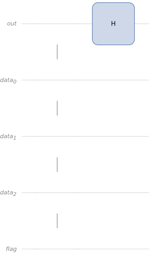
Find the probability of above quantum circuit. The first qubit corresponds to out register, next three corresponds to data registers and the last corresponds to flag register. Both the states are in uniform superposition state.
In[]:=
kk1[]["Probability"]
Out[]=
00000,10000
1
2
1
2
Check the amplitudes of all possible state of the above quantum circuit.
In[]:=
kk1[]["Amplitudes"]
Out[]=
00000,000010,000100,000110,001000,001010,001100,001110,010000,010010,010100,010110,011000,011010,011100,011110,10000,100010,100100,100110,101000,101010,101100,101110,110000,110010,110100,110110,111000,111010,111100,111110
1
2
1
2
Step 2 :Apply black box amp
Step 2 :Apply black box amp
In second step, we use a oracle amp to write the target amplitude to data registers controlled by the value in out register. The oracle when applied on the circuit prepared the system in the following state:
|〉(amp⊗I)|〉
ψ
1
ψ
0
i|0
ψ
1
1
M
M-1
∑
i0
〉
out
(n)
a
i
〉
data
〉
flag
where
ampiziz⊕
(n)
a
i
Create the amp oracle.
In[]:=
kk2=MapIndexed[QuantumOperator[{"C",alnToGate[#1],Splice[If[OddQ@First[#2],{{},{1}},{{1},{}}]]}]&,bin]
Out[]=
QuantumOperator,QuantumOperator


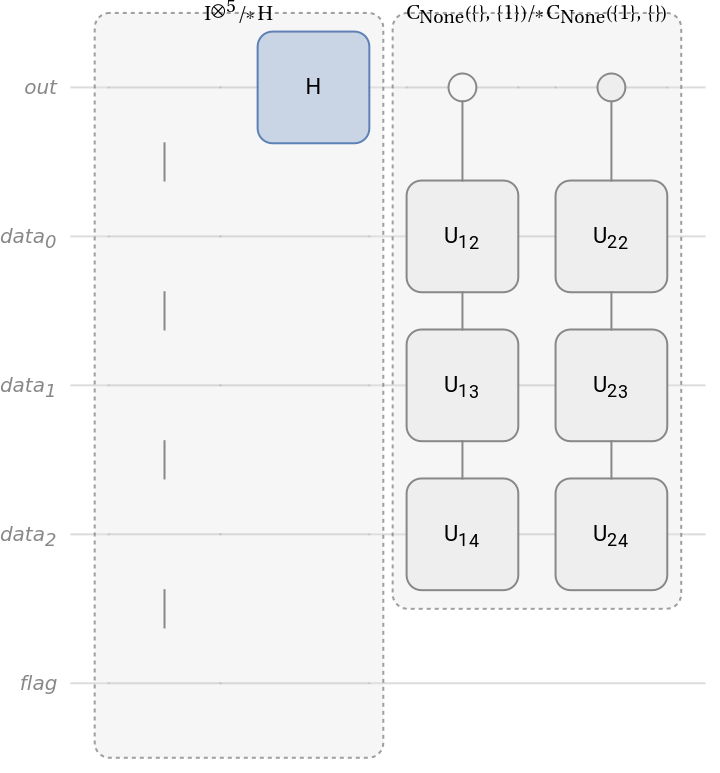
Create the quantum circuit operator created by the oracle. Note that the open-controlled gate are also used alternatively in the oracle
In[]:=
kk2op=QuantumCircuitOperator[kk2]
Out[]=
QuantumCircuitOperator
Check the full quantum circuit until the oracle amp is used.
In[]:=
kk2o=QuantumCircuitOperator[{kk1,kk2}]
Out[]=
QuantumCircuitOperator
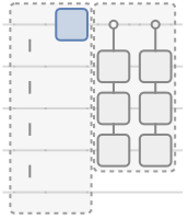
Visualize the diagram
In[]:=
kk2o["Diagram","WireLabels"->{"out","","","","flag"}]
data
0
data
1
data
2
Out[]=
Check the probability of above quantum circuit.
Note the differences between probability of both of the above quantum circuit.
Find the amplitudes of quantum circuit kk20.
Step 3 :Perform rotation operation
Step 3 :Perform rotation operation
A key contributor to the cost of Grover state preparation is the use of a subroutine called rot operator. to implement this procedure, the quantum computer would calculate θ, store the value in an ancillary register (flag) and use that register as the control for a sequence of rotation operations on the qubit. When applied to the system, it results in the following state.
Create the rot operator of the algorithm.
Create the quantum circuit operator from the rot operator.
Create the overall quantum circuit.
Visualize the circuit operator.
Note that the open controlled gate is used alternatively.
Check the probability of the quantum circuit formed yet.
Similary, find the amplitudes of the output of above quantum circuit.
Step 4: Perform amplitude amplification
Step 4: Perform amplitude amplification
Step 4a
Step 4a
Create phase oracle to be used in amplitude amplification.
Apply phase oracle function for the given input.
Create complete quantum circuit (until phase oracle)
Above circuit in dagger form is useful for the amplitude amplification.
Visualize the complete circuit in dagger form.
Step4b
Step4b
Create the Grover oracle excluding Hadamard gate.
Create the amplitude amplification oracle.
Visualize the oracle diagram.
Step 4c
Step 4c
Concatenate all steps together (including 2 rounds of amplitude amplification)
Visualize the diagram of the whole circuit.
Find the probability of states of above quantum circuit.
Check the amplitudes of states of above quantum circuit.
Step 5: Unprepare qubit wire used for precision
Step 5: Unprepare qubit wire used for precision
In the last step following amplitude amplification, we reset the data register by applying the amp oracle once more.
Check the probability and amplitudes of the complete quantum circuit (kk6)
data registers can now be discarded.
Step 6: Measure
Step 6: Measure
Verification
Verification
Check the probabilities of above quantum circuit.
Check the head of keys of the probabilities obtained above.
Convert the probabilities to string in little endian notation.
Extract selected states whose last qubit is 0 i.e. only flag register is taken into account.
Coming back to the initial input provided, data variable corresponds to the probability amplitudes. It was randomly chosen. In order to check the target amplitudes, it must be normalized and further squared to see the expected probability distribution. This will be be compared with the flag register probabilities.
Both counts obtained and expected values obtained has higher extent of match. This shows the capability of Grover state preparation algorithm. However, this approach would require over 11000 toffoli gates per round of amplitude amplification to prepare a quantum state. Many robust algorithm has been developed recently which brings this number(toffoli gates) down to many folds.
Initialization cells
Initialization cells
Function to returns the binary form upto ‘num’ bits of precision of the input decimal data.
Function to constructs the gate that corresponds to the input binary string X for bit ‘1’ and I for bit ‘0’.
References
References
CITE THIS NOTEBOOK
CITE THIS NOTEBOOK
Grover's state preparation algorithm
by Shivam Sawarn
Wolfram Community, STAFF PICKS, September 6, 2023
https://community.wolfram.com/groups/-/m/t/3007057
by Shivam Sawarn
Wolfram Community, STAFF PICKS, September 6, 2023
https://community.wolfram.com/groups/-/m/t/3007057