The Ising model is a fundamental mathematical framework for studying ferromagnetism and phase transitions. This computational essay explores the thermodynamic properties of 1D and 2D Ising models using the Metropolis-Hastings Markov chain Monte Carlo (MCMC) algorithm. By simulating spin configurations under periodic boundary conditions, macroscopic observables, such as internal energy, specific heat, and magnetization, are estimated across varying temperatures and magnetic fields. The MCMC results demonstrate exceptional agreement with exact analytical solutions, including Onsager’s analytical solution for the 2D phase transition. Ultimately, this project validates robust simulation methodologies that can be extended to model complex systems in physics, neuroscience, and sociology.
Introduction
Introduction
The Ising model, initially proposed by German physicist Wilhelm Lenz and solved in one dimension by his student Ernst Ising in 1925, is recognized as one of the most influential models in statistical mechanics for mathematically representing macroscopic behavior in interacting spin systems. It offers a mathematical framework for understanding how large-scale order emerges in systems of interacting spins. The model consists of a lattice of discrete spins, each interacting only with its nearest neighbors, and it captures the essential physics behind ferromagnetism, phase transitions, and critical phenomena. In the one-dimensional case, no phase transition occurs at finite temperature, yet the model still offers deep insight into how microscopic interactions give rise to macroscopic thermodynamic behavior. The two-dimensional model, unlike the one-dimensional model, undergoes a phase transition at a critical temperature, known as the Curie point.
Studying the 1D Ising model computationally offers multiple advantages: direct comparison between analytical solutions and simulation-based estimates is possible, making it an ideal system for validating Monte Carlo methods. The 2D model presents additional challenges, as it has a phase transition and more irregular thermodynamic behavior in comparison to the 1D model. In this project, simulation algorithms were developed and implemented for the 1D and 2D standard Ising models, using the Metropolis-Hastings method (a Markov chain Monte Carlo). It works by updating spins one at a time based on a local acceptance probability, allowing the system to evolve toward thermal equilibrium while sampling configurations according to the Boltzmann distribution. By repeatedly applying spin flips and these update rules, thermodynamic observables such as magnetization, energy, susceptibility, and heat capacity can be estimated as ensemble averages over generated spin configurations.
Using these simulations, this project studies how input parameters, specifically temperature, external magnetic field, and coupling constant, affect the observables of the system: internal energy, Helmholtz free energy, entropy, magnetization, specific heat, and spin-spin correlation functions/lengths. All simulations are conducted under periodic boundary conditions with a fixed lattice geometry, which isolates the effects of these parameters from other geometric variables. This simulation setup allows for a full investigation of how each parameter independently changes the system’s equilibrium properties.
Beyond its role in condensed matter physics and statistical mechanics, the Ising model’s mathematical structure has found incredible relevance in fields far from from magnetism. It underlies models of neural activity in computational neuroscience, the most notable being the Hopfield Network, as well as having applications in social dynamics, biology, and optimization. Developing robust simulation tools for the Ising model therefore serves two purposes: deepening understanding of magnetic phase transitions while also providing methodology applicable to a broad range of complex systems in computer science, sociology, and other fields.
1D Ising model
1D Ising model
Background
Background
The 1D Ising model represents a 1D chain of N spins with periodic boundary conditions with a total energy given by the Hamiltonian:
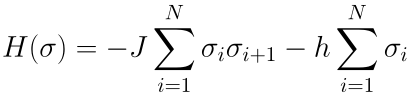
Where:


Metropolis-Hastings Implementation
Metropolis-Hastings Implementation
Define the Hamiltonian function:
hamiltonian[spins_,J_,h_]:=-J*Total[spins*RotateLeft[spins]]-h*Total[spins];
Define the magnetization function, which is just the sum of all the spins:
magnetization[spins_]:=Total[spins];
Define a function that computes the spin-spin correlation function by averaging the product of each spin with the spin sites away (using periodic boundary conditions) and subtracting the square of the mean spin.


spinSpinCorrFunction[spins_,r_]:=Mean[spins*RotateLeft[spins,r]]-Mean[spins]^2;
Define a single Metropolis-Hastings update step that randomly selects a spin , computes the energy change from flipping it (with periodic boundary conditions), and accepts the flip if or with probability otherwise.


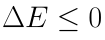

mhStep[state_,T_,J_,h_]:=With[{i=RandomInteger[{1,Length[state]}]},{dE=2.0*state[[i]]*(J*(state[[Mod[i-2,Length[state]]+1]]+state[[Mod[i,Length[state]]+1]])+h)},If[dE<=0.0||RandomReal[]<Exp[-dE/T],ReplacePart[state,i->-state[[i]]],state]];
Construct Metropolis-Hastings sweep by applying the single-spin update step times in succession, so that on average every spin in the lattice of length has one chance to flip.

mhSweep[state_,T_,J_,h_]:=Nest[mhStep[#,T,J,h]&,state,Length[state]];
Run a full 1D Ising Metropolis-Hastings simulation by initializing a random spin configuration of size , equilibrating it over a specified number of sweeps, then collecting a trajectory of post-equilibration sweeps to compute the mean internal energy , specific heat , mean absolute magnetization , magnetic susceptibility , and the spin-spin correlation function averaged over the trajectory for separations .
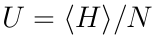

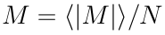


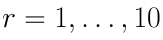
run1DIsingMH[nSpins_,T_,J_,h_,sweeps_,stats_]:=With[{initState=RandomChoice[{-1,1},nSpins]},{equil=Nest[mhSweep[#,T,J,h]&,initState,sweeps]},{traj=Rest[NestList[mhSweep[#,T,J,h]&,equil,stats]]},{energies=hamiltonian[#,J,h]&/@traj,mags=magnetization[#]&/@traj,absMag=Abs[magnetization[#]]&/@traj},<|"T"->T,"h"->h,"J"->J,"U"->Mean[energies]/nSpins,"C"->Variance[energies]/(T^2*nSpins),"M"->Mean[absMag]/nSpins,"Chi"->Variance[mags]/(T*nSpins),"PreEnergies"->energies,"PreMagnetizations"->mags,"CorrFunc"->Table[Mean[Mean[#*RotateLeft[#,r]]&/@traj],{r,1,10}]|>];
Set the simulation parameters, then run the 1D Ising Metropolis-Hastings simulation for every parameter pair in the grid while displaying a live progress indicator, and collect the results into a dataset.
nSpins=1000;sweeps=1000;stats=1000;jVal=1.0;tRange=Range[0.1,5.0,0.2];hRange={0.0,0.5,1.0};parameterGrid=Tuples[{tRange,hRange}];currSim=0;totalSims=Length[parameterGrid];results=Monitor[Map[(currSim++;run1DIsingMH[nSpins,#[[1]],jVal,#[[2]],sweeps,stats])&,parameterGrid],Row[{"Progress: ",ProgressIndicator[currSim,{0,totalSims}]," [",currSim," / ",totalSims," simulations complete]"}]];resData=Dataset[results];
Define the logarithm of the larger transfer-matrix eigenvalue, , used to compute the exact partition function and thermodynamic quantities for the 1D Ising model with periodic boundary conditions.

logEig1[b_,h_,J_]:=Log[Exp[J*b]*Cosh[b*h]+Exp[J*b]*Sqrt[Sinh[b*h]^2+Exp[-4*J*b]]];
Define the exact analytical thermodynamic quantities per spin derived from by differentiating with respect to and : magnetization , susceptibility , internal energy , specific heat , entropy , and free energy , then convert each from to temperature-dependent functions, and separately define the analytical correlation length .
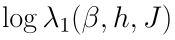

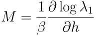
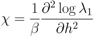
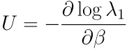
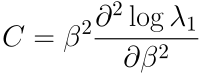

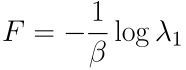
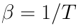

mDeriv[b_,h_,J_]=(1/b)*D[logEig1[b,h,J],h];chiDeriv[b_,h_,J_]=(1/b)*D[logEig1[b,h,J],{h,2}];uDeriv[b_,h_,J_]=-D[logEig1[b,h,J],b];cDeriv[b_,h_,J_]=b^2*D[logEig1[b,h,J],{b,2}];sDeriv[b_,h_,J_]=logEig1[b,h,J]+b*uDeriv[b,h,J];fDeriv[b_,h_,J_]=-(1/b)*logEig1[b,h,J];mAnalytical[T_,h_,J_]:=mDeriv[1/T,h,J];chiAnalytical[T_,h_,J_]:=chiDeriv[1/T,h,J];uAnalytical[T_,h_,J_]:=uDeriv[1/T,h,J];cAnalytical[T_,h_,J_]:=cDeriv[1/T,h,J];sAnalytical[T_,h_,J_]:=sDeriv[1/T,h,J];fAnalytical[T_,h_,J_]:=fDeriv[1/T,h,J];xiAnalytical[T_,J_]:=-1/Log[Tanh[J/T]];
Filter the specific heat data with a zero magnetic field from the simulation results data, then calculate entropy via thermodynamic integration by interpolating , then integrate it numerically from the lowest sampled temperature using , and separately generate the corresponding analytical specific heat curve at for comparison.

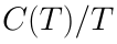
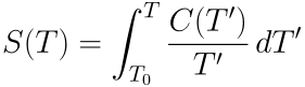
cDataH0=SortBy[{#T,#C}&/@Select[Normal[resData],#h==0.0&],First];sThermoIntData=Module[{tValues,cValues,integrand,interp,antideriv,cIntegrated},tValues=cDataH0[[All,1]];cValues=cDataH0[[All,2]];integrand=cValues/tValues;interp=Interpolation[Transpose[{tValues,integrand}],InterpolationOrder->3];antideriv=Derivative[-1][interp];cIntegrated=(antideriv/@tValues)-antideriv[tValues[[1]]];Transpose[{tValues,cIntegrated}]];plotCH0=Values/@Normal[resData[Select[#["h"]==0.0&],{"T","C"}]];analyticalCData=Table[{T,cAnalytical[T,0.0,jVal]},{T,tRange}];
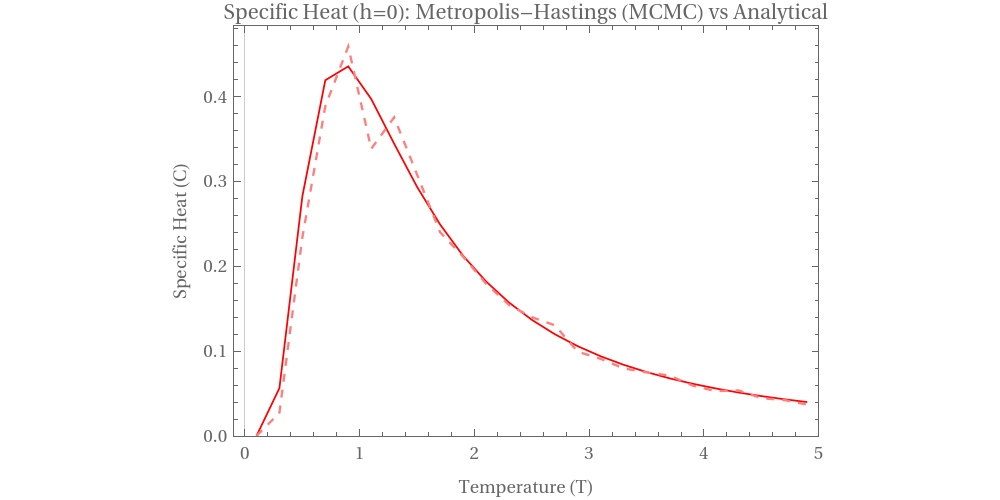
Plot of the analytical and MCMC specific heat curves as a function of temperature at zero magnetic field , using solid and dashed red lines respectively.
p1=ListLinePlot{analyticalCData,plotCH0},


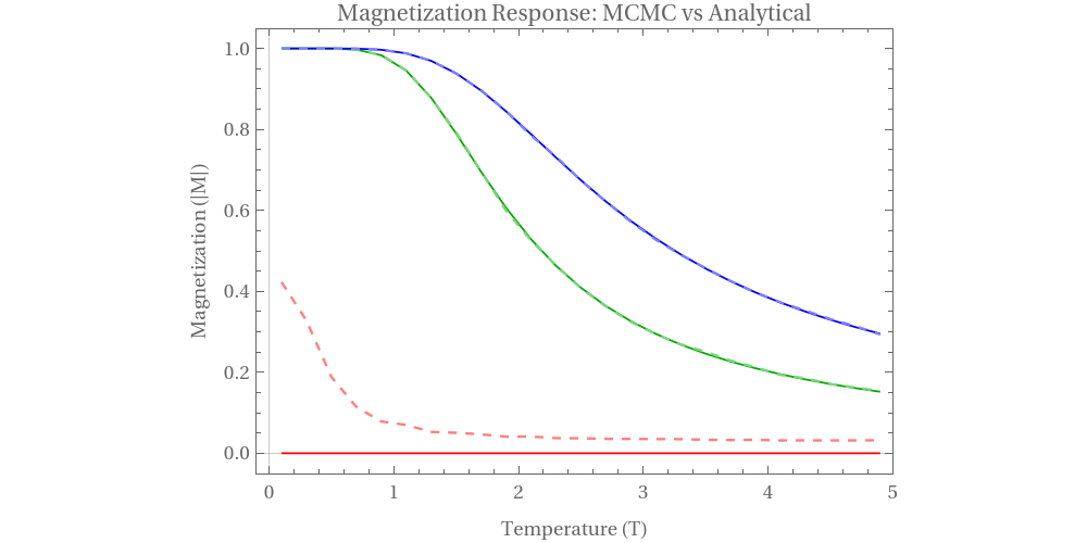
Filter magnetization data from the simulation results and generate the corresponding analytical magnetization curves for each field value in , across all three magnetic field strengths .
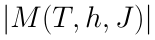
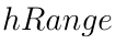
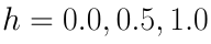
plotM=Table[Values/@Normal[resData[Select[#["h"]==hVal&],{"T","M"}]],{hVal,hRange}];analyticalMData=Table[{T,hVal,Abs[mAnalytical[T,hVal,jVal]]},{hVal,hRange},{T,tRange}];p2=ListLinePlotJoin[analyticalMData,plotM],
One thing to notice about the fit is that when , the MCMC predicted solution does not fit the analytical solution due to finite chain size and the fact that this is absolute magnetization.


Finds the temperature closest to 2.1 in the simulation data for the h=0 field case, filter out the sampled pre-equilibrium energy values recorded at that temperature, and compute the corresponding analytical mean energy as a comparison, then plot a histogram of the sampled energies with a vertical red line marking the analytical mean energy.
In this plot, lattice distance and temperature affect spin-spin correlation, or how two spins separated from each other can affect each others’ spins. The MCMC simulations are tested at two temperatures.
Correlation length represents the average distance by which fluctuations of spins are correlated with one another. This plot compares the analytical solution for the correlation length with the MCMC predicted correlation length.
2D Ising model
2D Ising model
Background
Background
Metropolis-Hastings Implementation & Checkerboard Decomposition
Metropolis-Hastings Implementation & Checkerboard Decomposition
Define the Hamiltonian in 2D, with vertical and horizontal contributions to the first summation
Define the total magnetization, which is just the sum of all the spins in the lattice
Neighbor-summing function
The even and odd grids are for the Checkerboard Decomposition, where each grid only holds spins of one color, and depends on the other grid to update:
Metropolis-Hastings function for single iteration
Metropolis-Hastings function for a sweep (multiple iterations)
Analytical solution for the critical temperature:
Onsager’s analytical solution for magnetization, internal energy, and specific heat
Size of the domain, sweeps, J value:
Simulation function, along with a counter and progress bar:
Plot for spontaneous magnetization, and a comparison between the analytical solution and the MCMC predicted solution
Plot of internal energy, comparing MCMC and Onsager analytical solution
Plot of specific heat, and it diverges as T approaches the critical temperature (2.269):
This is a plot to see how with three different temperatures, how the spin-spin correlation changes as the distance between two spins increases:
Conclusion
Conclusion
In this project, I implemented the Metropolis-Hastings algorithm for simulating 1D & 2D Ising models, and optimized the 2D algorithm using checkerboard decomposition. The simulations exhibit incredible accuracy and computational efficiency, and plots were generated to understand the effects of varying different input variables of the Ising model. Specific heat, internal energy, spin-spin correlation, magnetization, and various other thermodynamic properties of the Ising model were studied, and the Metropolis-Hastings algorithm successfully adhered to the analytical solutionsof both the 1D and 2D system.
Future Directions
Future Directions
Some future areas of study in simulation of Ising models are in generalized Ising models, which are Ising models with expansions to such as more spin states, more complex spin-spin interactions, and changes in lattice geometry. More complex mathematical methods may be needed for simulating generalized Ising models, as more spin states can lead to a larger configuration space, making it harder to compute partition functions analytically. Additionally, complex spin-spin interactions can introduce which can cause conventional Monte Carlo algorithms to suffer from severe critical slowing down. An interesting frontier in the simulation of Ising models is in Machine Learning (ML), as ML algorithms can be trained on Monte Carlo simulations to predict thermodynamic properties directly from data. These ML methods could potentially speed up Ising model simulations, and would give us a better understanding of complex phenomena in fields beyond physics that use Ising-type models, such as computational neuroscience (modeling neural networks and brain activity), sociology (modeling opinion dynamics and social behavior), and biology (modeling gene regulatory networks and collective cell behavior).
References
References
◼
Ising model:
Ising model. (n.d.). In Wikipedia. Retrieved July 9, 2026, from https://en.wikipedia.org/wiki/Ising_model
Ising model. (n.d.). In Wikipedia. Retrieved July 9, 2026, from https://en.wikipedia.org/wiki/Ising_model
◼
Metropolis–Hastings algorithm:
Metropolis–Hastings algorithm. (n.d.). In Wikipedia. Retrieved July 9, 2026, from https://en.wikipedia.org/wiki/Metropolis%E2%80%93Hastings_algorithm
Metropolis–Hastings algorithm. (n.d.). In Wikipedia. Retrieved July 9, 2026, from https://en.wikipedia.org/wiki/Metropolis%E2%80%93Hastings_algorithm
◼
Gautam. (2024). Using Metropolis Hastings on the Ising model [Course notes]. Carnegie Mellon University, Department of Mathematical Sciences. https://www.math.cmu.edu/~gautam/c/2024-387/notes/06-metropolis-hastings.html
◼
Lipowski, A. (2022). Ising model: Recent developments and exotic applications. Entropy, 24(12), 1834. https://doi.org/10.3390/e24121834
◼
Anthropic. (2026). Claude (Sonnet 5.0) [Large language model, used for generating code] https://claude.ai
Acknowledgements
Acknowledgements
I would like to thank my mentor, Dan McDonald for his guidance on my project, and my advocate Dr. Madeleine Sutherland for strengthening my Wolfram Language skills and helping me develop this project idea. I would also like to thank Lucas Squillante and Rafael Caballero for their help on understanding Ising models, the underlying math, and the scope of my project. I’m especially thankful to Megan, Eryn, Rory, Anne, and to Stephen Wolfram for introducing me to Wolfram Language, for their guidance, and for giving me this project. Finally, thank you to Eric Archerman, Bryan Chen, and Arnay Garhyan for being great teaching assistants throughout the program.
Additional thanks to Stephen Wolfram for suggesting this project.
CITE THIS NOTEBOOK
CITE THIS NOTEBOOK
Metropolis-hastings simulations of The Ising model: ferromagnetism and phase transitions
by Nikhil Srinivasan
Wolfram Community, STAFF PICKS, July 12, 2026
https://community.wolfram.com/groups/-/m/t/3753457
by Nikhil Srinivasan
Wolfram Community, STAFF PICKS, July 12, 2026
https://community.wolfram.com/groups/-/m/t/3753457