Iran MO 2019 Geometry Problem
In[]:=
<<MaTeX`
MaTeX//Framed
Out[]=
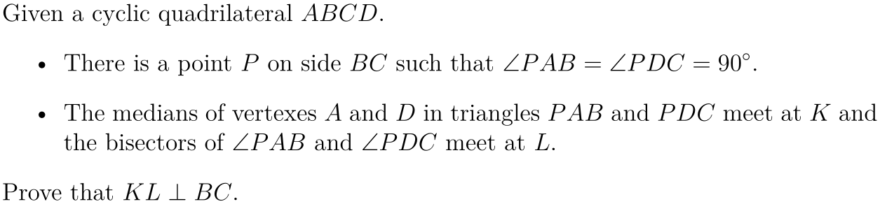
gs=GeometricScene,{GeometricAssertion[Style[Polygon@{a,b,c,d},Transparent],"Cyclic"],PlanarAngle[{b,a,p}]PlanarAngle[{p,d,c}]90Degree,Line[{b,p,c}],mMidpoint[{b,p}],nMidpoint[{p,c}],Line[{a,m,k}],Line[{d,n,k}],l∈TriangleConstruct[{p,a,b},{"AngleBisector",a}],l∈TriangleConstruct[{p,d,c},{"AngleBisector",d}],Line[{k,l}],EuclideanDistance[a,d]2.7}//RandomInstance[#,RandomSeeding9]&;
Plot with some boundary
In[]:=
Show[gs["Graphics"],PlotRange{-2.5,1.4}]
Out[]=
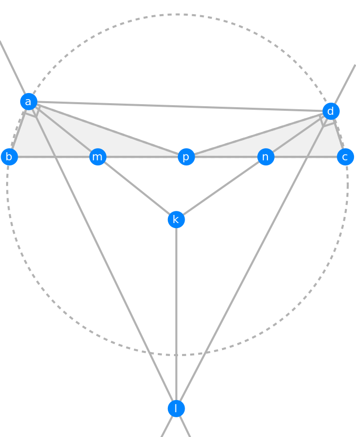
Mathematica automatically finds the conclusion
In[]:=
FindGeometricConjectures[gs,GeometricAssertion[__,"Perpendicular"]]["Conclusions"]
Out[]=
{GeometricAssertion[{Line[{b,m,p,n,c}],Line[{l,k}]},Perpendicular],GeometricAssertion[{Line[{d,c}],Line[{p,d}]},Perpendicular],GeometricAssertion[{Line[{a,p}],Line[{b,a}]},Perpendicular]}
In[]:=
%[[1]]
Out[]=
GeometricAssertion[{Line[{b,m,p,n,c}],Line[{l,k}]},Perpendicular]
Proof
Proof
If you take a look at the diagram and focus on triangle ABP and CPD, it is almost like the upper part of the configuration in butterfly theorem
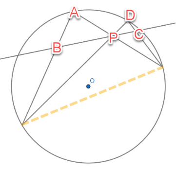
Naturally, we just want to extend the lines of AB, CD, AP and DP. Let AB and DP intersect at E, DC and AP at F. Connect EF. Use the intersection function used across several community articles to find the cross point of my extensions.
In[]:=
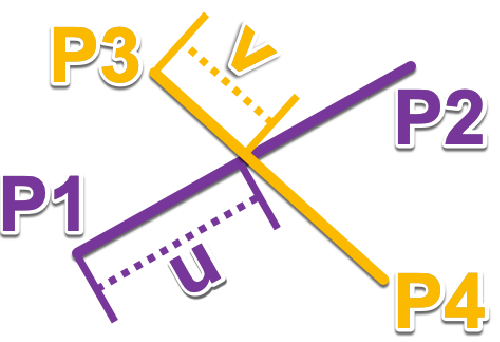
segmentIntersection[p1_List,p2_List,p3_List,p4_List]:=Block[{u,v},Module[{sol},sol=Solve[u*(p2-p1)+p1v*(p4-p3)+p3,{u,v}];{u,v,u*(p2-p1)+p1}/.sol〚1〛]]
For convenience, let’s add some variable to store the numerical values for my points
In[]:=
{ptA,ptB,ptC,ptD,ptP,ptK,ptL,ptM,ptN}={a,b,c,d,p,k,l,m,n}/.gs["Points"];
Use the function above and find the exact location of E and F
In[]:=
ptE=segmentIntersection[ptA,ptB,ptD,ptP]〚3〛;ptF=segmentIntersection[ptD,ptC,ptA,ptP]〚3〛;
Also the following utility function helps me to put the new points back into the diagram with the same style as the auto generated labels in GeometricScene.
In[]:=
assoPts=;
In[]:=
label[str_String]:=With[{pos=assoPts[str]},{PointSize[0.045],Hue[0.58,1,1],Point[pos],Text[Style[str,White,12],pos]}]
If you want to add auxiliary lines onto the diagram, you do not have to generate the geometric scene again. Simply call the “Graphics” attribute from the geometric scene object. Then use Show to add a layout of added lines on top of the geometric scene graphics.
In[]:=
Show[Graphics[{{Dashed,Blue,HalfLine[{ptA,ptB}],HalfLine[{ptD,ptC}],HalfLine[{ptA,ptP}],HalfLine[{ptD,ptP}],Line[{ptE,ptF}]}}~Join~(label/@{"e","f"})],gs["Graphics"],PlotRange{{-1,4},{-2.5,1.4}}]
Out[]=
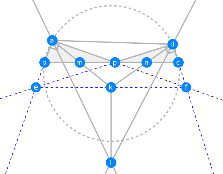
Because Mathematica draws the diagram to a very high precision, we can observe that E-K-F being collinear is really not just lucky or error. Perhaps it is something we can prove later. To verify the observation, lets compute the angle EKF
In[]:=
RowRound,°
PlanarAngle[{ptE,ptK,ptF}]
Degree
Out[]=
180°
Other the hand, after extensions of some lines and obtain the intersections, we can see the quadrilateral AEFD is quite special. We can HatchFilling function introduced in V12 to gently highlight the region.
In[]:=
Show[Graphics[{{Opacity[0.9],Green,HatchFilling[],EdgeForm[Dashed],Polygon[{ptA,ptE,ptF,ptD}]},Dashed,Thickness[0.003],Line[{ptA,ptF}],Line[{ptD,ptE}],Line[{ptB,ptC}],label/@{"e","f"}}],gs["Graphics"]]
Out[]=
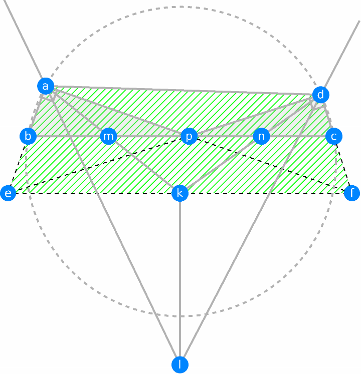
Because we are given angle AEF and EDF are both right angle, we can conclude immediately AEFD is cyclic. Additionally, not like regular concyclic quadrilateral, we have the inscribed angle equal to 90 degree. This tells us that EF is the diameter of the circumcircle which goes through points A, E, F and D.
The other useful result we have from cyclic quadrilaterals is that angle EAD plus DFE is 180 degree. But we are also given ABCD is cyclic, angle EAD plus DCB is 180 degree. Therefore angle BCD equals to angle DFE. Notice these two angles are corresponding angles of lines CB and EF and transversal DF. Thus CB and EF are parallel lines. Lets check the result numerically by vector relations
The parallel relation implies that triangle ABP and AEF are homothety. Because M is the middle point of BP, AM must intersect at the mid point of EF. Similarly, DN meets EF at the mid point of EF. It is clear that this K is the mid point of EF due to the concurrency of the three lines. Which also prove that EKF collinear.
The last part is similar to finding K. We know that AL is angular bisector of angle EAF, so AL meets arc EF at its mid point L’ by inscribed angle theorem. Also DL must pass L’. Thus L’ is where AL and DL meet. So L is L’.
Eventually, this KL is just a link between center K of semicircle (arc) ELF and the mid point point of the arc.
Of course, KL is perpendicular to line E-K-F
Of course, KL is perpendicular to line E-K-F
Animation
Animation
To efficiently animate the diagram in our problem, we need to rethink the process above. With the given conditions in the problem, we know that ABCD being cyclic is the sufficient and necessary condition for cyclic AEFD. Thus, we can safely parameterize the components as such
◼
K as (0,0)
◼
EK = KF = 2 as radius of circle K
◼
A and D on circle K in trig form
Then we can construct all required points without solving equation like in geometric scene. You can play with animation by dragging the sliders without any delay.
Remark
Remark
◼
Use GeometricScene to construct the diagram synthetically
◼
Use inscribed angle theorem to find cyclic quadrilaterals
◼
Use relations in cyclic quadrilateral to find parallel lines
◼
Use Manipulate to create a forward simulation without simple parametric equation of circle