Dutch Railway Network
Dutch Railway Network
The Dutch railway network is one of the densest and most connected rail systems in Europe. It connects nearly all major Dutch cities and towns while also providing international connections to neighboring countries. Graph theory provides the perfect tool for analyzing this network, allowing us to better understand its structure, connectivity, robustness, and the role that individual stations play within the transportation system.
Graph representation
Graph representation
Analysis
Analysis
Vertex and Edge Count
Vertex and Edge Count
The resulting graph consists of 404 vertices (stations) and 440 edges (direct railway connections).
We can calculate the number of vertex with the command:
In[]:=
VertexCount[DRN]
Out[]=
404
We can calculate the number of edges with the command:
In[]:=
EdgeCount[DRN]
Out[]=
440
This is actually the first step in analyzing any graph. The total number of vertices (also known as the order) and the total number of edges (also known as the size) provide fundamental information about the structure of a graph or network.
Municipalities - Another small side note
Vertex Degree
Vertex Degree
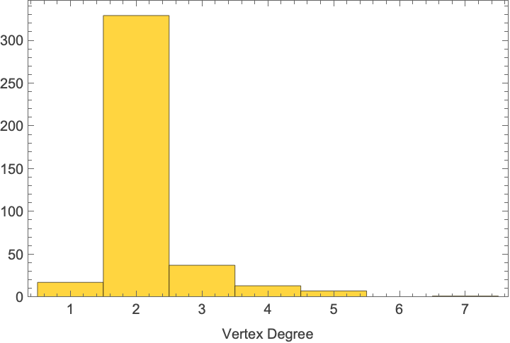
As we saw, this network has 404 vertices (stations) and 440 edges (direct railway connections), from which we can already see that the network is relatively sparse. In other words, not every station is directly connected to many others, and most stations are only linked to a limited number of nearby stations. This is consistent with the fact that most stations are connected to only a small number of other stations, which can be seen more clearly through the vertex degree histogram and the mean vertex degree.
We can calculate the vertex degree with the command:
In[]:=
VertexDegree[DRN]
Out[]=
{2,3,3,2,2,2,2,2,2,2,3,2,2,2,2,3,2,2,2,2,2,2,2,2,2,3,2,2,2,2,5,2,2,2,2,2,3,3,2,2,2,3,2,2,2,2,3,2,2,4,2,2,2,2,2,2,2,2,2,2,2,3,2,2,2,2,5,2,2,2,2,2,3,2,2,2,1,3,2,2,2,4,2,2,2,2,2,2,2,2,5,2,2,2,2,2,2,2,2,2,3,2,2,2,2,2,2,2,1,5,2,2,2,2,2,2,2,2,2,2,2,3,5,2,2,2,2,3,2,3,3,2,2,7,2,2,2,2,2,2,2,2,2,5,2,3,2,2,2,2,2,2,3,2,2,2,2,3,2,3,2,2,3,2,3,3,4,2,2,2,4,2,4,2,2,2,2,2,3,2,1,2,2,2,2,2,2,2,1,2,2,2,1,2,2,2,2,2,2,2,2,2,5,2,2,2,2,2,2,2,2,2,2,2,3,2,2,1,2,2,2,3,2,2,2,2,2,2,4,4,2,2,2,3,4,2,2,2,2,2,2,2,2,2,2,2,2,2,2,2,2,2,2,2,4,2,2,3,2,2,2,2,2,2,4,2,2,2,2,2,2,2,2,2,2,2,2,2,2,2,2,4,4,2,2,2,2,2,2,2,2,3,2,2,2,2,2,2,2,2,2,2,2,2,2,2,2,2,2,2,3,2,3,2,2,3,2,2,2,2,1,2,2,2,4,2,2,2,2,2,2,2,2,2,3,3,2,2,1,2,2,2,2,3,2,2,2,2,2,2,2,2,2,2,2,2,2,2,2,2,2,2,2,2,2,2,3,2,2,2,2,2,2,2,2,1,1,1,2,2,2,2,2,2,2,2,2,2,2,1,2,2,1,2,2,2,2,1,2,2,1,1,2,1}
And we can visualize the vertex degree histogram as:
In[]:=
Histogram[VertexDegree[DRN],PlotRange->All,FrameLabel->{"Vertex Degree"},Frame->True]
Out[]=
We can also calculate the mean vertex degree as:
In[]:=
Mean[VertexDegree[DRN]]//N
Out[]=
2.17822
In this case, the mean vertex degree of about 2.17 indicates that most stations are connected to roughly two other stations. This suggests that the network is largely structured as a collection of line-like segments rather than a highly interconnected system, as one might otherwise expect. Additionally, it is interesting to identify that the station with the largest number of connections is Zwolle:
In[]:=
VertexList[DRN][[PositionLargest[VertexDegree[DRN]]]]
Out[]=
{Zwolle}
The fact that most stations are connected to roughly two other stations may not be immediately intuitive, but it becomes clearer when considering how direct rail connections actually work. As an example, one can travel from Amsterdam Sloterdijk to Haarlem on a direct train, but the route still passes intermediate stations (even if the train does not stop there), such as Halfweg and Haarlem Spaarnwoude. This shows that even when two major stations appear closely connected, the actual network structure still includes intermediate stations along the way. As a result, major stations such as Amsterdam Sloterdijk can appear less connected in practice.
Weights
Weights
Edge Weights
As we can see from the edge weights (representing distances), the distances between stations are generally not very large, as shown in the histogram of edge weights:
Out[]=
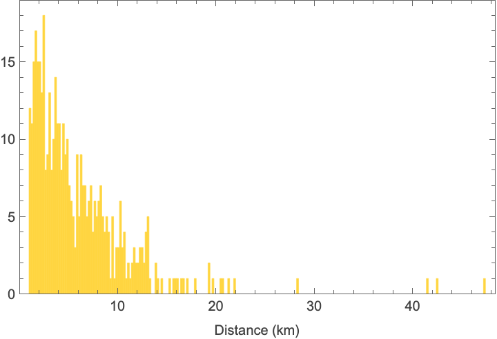
This is because, as we mentioned before, even when two major stations appear closely connected, the actual network structure still includes intermediate stations along the way, which reduces the distances between directly connected stations.
Vertex Weights
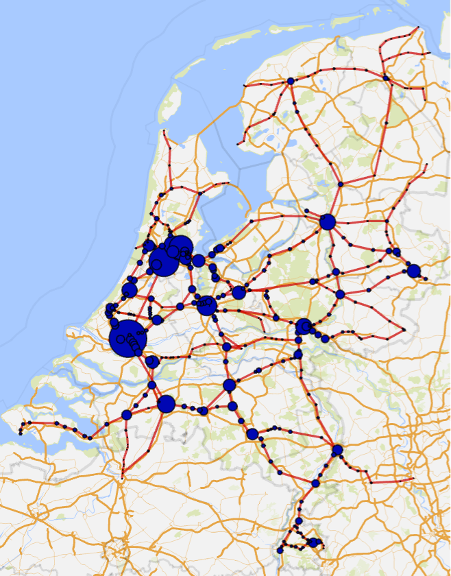
For the vertex weights (representing the number of disruptions):
Out[]=
We can look at the histogram of the number of disruptions:
In[]:=
Histogram[Values[DRNVW],200,PlotRange->All,FrameLabel->{"Disruptions"},Frame->True]
Out[]=
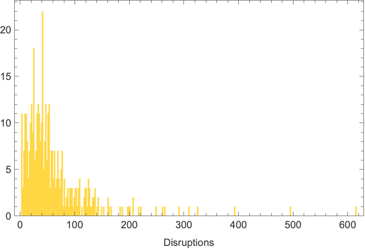
The histogram shows how certain stations have significantly higher values. The top 10 stations with the largest number of disruptions include:
In[]:=
DRNVW[[Flatten[PositionLargest[Values[DRNVW],10]]]]
Out[]=
{Rotterdam Centraal614,Schiphol Airport494,Amsterdam Centraal392,Utrecht Centraal325,Amsterdam Sloterdijk308,Breda290,Arnhem Centraal265,Zwolle261,Leiden Centraal248,Amersfoort Centraal221}
Distance
Distance
To analyze the distances in our graph we can use the graph distance matrix (often referred to as the “distance matrix”). The distance matrix is a square matrix that represents the pair-wise distances between vertices. Each entry in the matrix specifies the shortest path distance between two vertices, that represents the number of edges connecting the two vertices.
We can calculate the GraphDistanceMatrix with the command:
In[]:=
DM=GraphDistanceMatrix[DRN];
With the distance matrix, we can find the longest distance between any two vertices in the graph:
In[]:=
Max[DM]
Out[]=
57
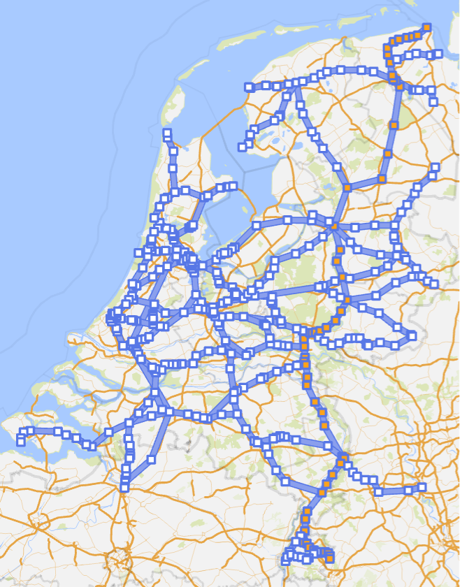
The longest distance of 57 suggests that it takes 59 stops (including transfers) to travel between the most distant vertices in the network. This is consistent with the structure of the Dutch railway system, where intercity trains are designed to connect major hubs while bypassing many intermediate stops. This allows longer-distance travel to remain relatively efficient, even if the underlying graph includes many local connections. In this case, the longest travel path based on the number of stations is from “Kerkrade Centrum” to “Eemshaven”:
In[]:=
VertexList[DRN][[Position[DM,Max[DM]][[1]]]]
Out[]=
{Kerkrade Centrum,Eemshaven}
And we can visualize this route (from Kerkrade Centrum to Eemshaven) on the map:
sp=FindShortestPath[Graph[ResourceData["Dutch Railway Network"],EdgeWeight->ResourceData["Dutch Railway Network","EdgeWeight"]],"Kerkrade Centrum","Eemshaven"];
Out[]=
Graph Partition
Graph Partition
A graph partition is a division of the vertices of a graph into subsets or components, where each subset forms a connected subgraph. It involves breaking a graph into smaller parts; in the railway system, this can reveal clusters of stations that are related or share similar characteristics. For instance, stations within the same partition may lie on the same railway line or exhibit similar passenger usage patterns. One possible graph partition of the dutch railway network is:
This partition is somewhat consistent , grouping together the major cities and the most highly connected stations, while separating them from regions that are still important but generally less visited and less densely connected.
Graph Communities
Graph Communities
Graph communities, also known as network communities, refer to subsets of vertices within a larger network that exhibit higher levels of interconnectedness or similarity among themselves compared to nodes outside of those subsets. For this graph the communities turn out to be:
These graph communities can represent clusters of stations that have strong connections or similar characteristics. For instance, stations within the same community often belong to the same railway lines.
Eccentricity
Eccentricity
The eccentricity of a vertex is the maximum distance from that vertex to all the other vertices in the network. If the eccentricity of a vertex is small, then all the other vertices are close to that vertex. Conversely, if the eccentricity is large, then all the other vertices are far away. So, we can calculate the vertex eccentricity for each vertex and determine how far away each vertex is from the others:
The diameter of a graph is the maximum eccentricity. This definition is intuitive because when two nodes are as far apart as possible, they must be placed at the diametrically opposite ends of the network.
We can calculate the graph diameter with the command:
The nodes with eccentricity equal to the diameter are the vertices farthest away; this is the periphery of a graph. In the railway context, these could be stations located farther away.
We can find the graph periphery with the command:
In this case the periphery nodes are “Kerkrade Centrum” and “Eemshaven”.
The radius of a network is the minimum eccentricity.
We can calculate the graph radius with the command:
And,the nodes with eccentricity equal to the radius are the center of the graph.
We can find the graph center with the command:
In this case the center node is “Arnhem Zuid”.
Centrality
Centrality
Centrality helps to identify which nodes are the most influential or central in terms of communication, information flow, or connectivity within the network. There are different centrality metrics, each capturing a different aspects. The choice of metric depends on the type of insight being sought. In a railway system, degree centrality (also know as vertex degree), closeness centrality, and betweenness centrality are particularly informative, as they highlight interchange stations, accessibility, and transfer dependency patterns.
Closeness Centrality
Closeness centrality is a network metric that measures how close a node is to all other nodes in a network on average. It quantifies how quickly or easily information or influence can spread from a particular node to other nodes in the network.
We can find the closeness centrality of each vertex with the command:
We can visualize the closeness centrality in a histogram:
In this context, stations with high closeness centrality are close to many other stations in terms of travel distance or travel time, indicating that they are among the most important stations in the network and likely require a higher frequency of trains passing through them.
Betweenness Centrality
Betweenness centrality is a network metric that measures the extent to which a node in a network acts as a bridge or intermediary between other nodes. It quantifies how often a particular node lies on the shortest paths between pairs of other nodes in the network.
We can find the betweenness centrality of each vertex with the command:
We can visualize the betweenness centrality in a histogram:
In the subway context, stations with high betweenness centrality act as critical transfer points and are crucial for the overall flow of passengers in the network. This can help identify stations where disruptions should be especially avoided, since problems at these locations can affect large parts of the network:
Postman Tour
Postman Tour
The postman tour, also known as the Chinese Postman Problem, identifies the shortest route that traverses every edge in the graph at least once. In this context, it can be interpreted as the ideal route for travelling through the entire railway network while covering every railway connection at least once:
We can compute the postman tour with the command:
And we can visualize it:
If one wanted to visit every station while taking the shortest possible route needed to traverse the entire railway system, the total distance traveled would be about 3492.58 km.
To put this into perspective, travelling that distance from Amsterdam would already take you as far as Turkey, as illustrated by the circle with a radius of 3492.58 km centered on Amsterdam Central:
On disruptions
On disruptions
Degree Centrality
One of the observations we can make is that stations with the highest vertex degree (which can also be interpreted as degree centrality), and which function as key junctions where multiple lines meet, include stations such as Zwolle, Amsterdam Sloterdijk, Rotterdam Centraal, Utrecht Centraal, and Amersfoort Centraal:
Many of these stations also appear in the list of 25 stations with the highest number of disruptions:
The overlap between both sets is:
Only a few stations fall outside this overlap:
The relatively large overlap is expected, since these stations handle a high volume of frequent services, which increases the likelihood of delays and operational issues. In this sense, vertex degree can be interpreted as a partial proxy for congestion, since highly connected stations tend to concentrate traffic from multiple lines. However, even with this overlap, it is important to remember that vertex degree should only be used as a first approximation when identifying stations that may be more prone to disruptions. It helps highlight parts of the network that require attention, but it does not fully explain disruption patterns on its own. To find disruption patterns we should also consider other parts of the network, since some stations may have high connectivity without experiencing many disruptions, while others may be operationally sensitive for reasons not captured by network structure alone.
Betweenness Centrality
On the other hand, betweenness centrality highlights a slightly different role. As we saw, stations such as Zwolle, Breda, Rotterdam Centraal, Deventer, and Amersfoort Centraal have high betweenness centrality because many shortest paths in the network pass through them. This means that these stations act as bridges between different parts of the country, so disruptions at these locations can have a relatively large impact on overall connectivity. This naturally raises the question of how strongly this structural importance is related to observed disruptions:
The overlap with stations that experience many disruptions is:
And the remaining stations in the betweenness list are:
The overlap is therefore not very large. This suggests that high betweenness centrality does not automatically imply a high number of disruptions.
But, one observation we can make is that a small group of stations; like Zwolle, Breda, Utrecht Centraal, Amersfoort Centraal, Rotterdam Centraal, and Duivendrecht; appears consistently across all three measures. This suggests that they are not only well connected, but also structurally important and frequently used within the network. Zwolle (marked in red) is particularly notable in this context. Despite not being one of the largest cities in the Netherlands, it emerges as one of the most central stations, reflecting its strategic position as a national railway hub connecting the northern and eastern regions with the Randstad and the south.
Conclusion
Conclusion
Graph theory metrics can help optimize railway network design, identify critical transfer points, and improve the overall efficiency of the network. For example, they can help highlight which stations are more prone to disruptions, as we saw that stations with larger vertex degree are often linked to the most disruption-prone parts of the network. This makes vertex degree a useful first indicator for identifying important lines and stations that should be maintained carefully to reduce the risk of large-scale disruptions.
One possible idea that emerges from this analysis is that some of these highly disruption-prone areas could benefit from alternative routes or additional railway connections that reduce their dependency on a single hub. In this way, when disruptions occur, passenger flow could be redistributed more easily through other parts of the network, helping to reduce the impact of large-scale disruptions.
Bibliography
Bibliography
1
.“Gemeentelijke herindeling” [Municipal reorganisation] (in Dutch). Government of the Netherlands. 21 December 2022. Retrieved 2 January 2023. https://www.rijksoverheid.nl/onderwerpen/gemeenten/gemeentelijke-herindeling
2
.“Municipalities of the Netherlands.” Wikipedia. Accessed May 26, 2026. https://en.wikipedia.org/wiki/Municipalities_of_the_Netherlands
3
.Wolfram Data Repository. Dutch Railway Network. Wolfram Discrete Computation (2025). https://datarepository.wolframcloud.com/resources/Dutch-Railway-Network/
4
.Rijden de Treinen. Train Disruptions Dataset. All train disruptions in 2023.. https://www.rijdendetreinen.nl/en/open-data/disruptions
5
.Rijden de Treinen. Railway Stations Dataset. Dutch and international railway stations as of September 2023. https://www.rijdendetreinen.nl/en/open-data/stations
CITE THIS NOTEBOOK
CITE THIS NOTEBOOK
Analysis of the Dutch railway network Using graph theory
by Alejandra Ortiz Duran
Wolfram Community, STAFF PICKS, May 26, 2026
https://community.wolfram.com/groups/-/m/t/3722625
by Alejandra Ortiz Duran
Wolfram Community, STAFF PICKS, May 26, 2026
https://community.wolfram.com/groups/-/m/t/3722625