ABSTRACT (original article): The mechanics of a foam depends on bubble shape, bubble network topology, and the material at hand, be it metallic or polymeric, for example. While the shapes of bubbles are the consequence of minimizing surface area for a given bubble volume in a space-filling packing, if one were to consider biological tissue as a foam-like material, the zoology of observed shapes of cells perhaps motivates different energetic contributions. Building on earlier two-dimensional results, here, we focus on a mean field approach to obtain the elastic moduli for an ordered, three-dimensional vertex model. We use the space-filling shape of a truncated octahedron and an energy functional containing a restoring surface area spring and a restoring volume spring. The tuning of the three-dimensional shape index exhibits a rigidity transition via a compatible–incompatible transition. Specifically, for smaller shape indices, both the target surface area and volume cannot be achieved, while beyond some critical value of the three-dimensional shape index, they can be, resulting in a zero-energy state. In addition to analytically determining the location of the transition in mean field, we find that the rigidity transition and the elastic moduli depend on the parameterization of the cell shape. This parameterization effect is more pronounced in three dimensions than in two dimensions given the zoology of shapes that a polyhedron can take on (as compared to a polygon). We also uncover nontrivial dependence of the elastic moduli on the deformation protocol in which some deformations result in affine motion of the vertices, while others result in nonaffine motion. Such dependencies on the shape parameterization and deformation protocol give rise to a nontrivial shape landscape and, therefore, nontrivial mechanical response even in the absence of topology changes. CITATION (original article): Kyungeun Kim et al 2024, Mean-field elastic moduli of a three-dimensional, cell-based vertex model, New J. Phys. 26 043009. https://doi.org/10.1088/1367-2630/ad3099
Introduction
Introduction
Imagine looking at the world around us through a microscope. You’d see that many materials - from soap bubbles to metal structures to living tissues - are made up of tiny units that fit together perfectly to fill space. Just like a box of perfectly packed oranges, these units must have specific shapes to fill space without gaps.
Some of these space-filling shapes are familiar, like cubes. Others might be less familiar, like dodecahedra (12-sided shapes) and truncated octahedra (14-sided shapes). What’s special about these shapes is that they’re all convex, meaning they have no dents or caves - think of shapes that could hold water without any leaks.
Scientists have been studying how these shapes work together, especially in living systems. In the 1980s, Honda and his team pioneered this research by looking at how cells arrange themselves in two dimensions - imagine cells squished between two glass slides. This helped them understand processes like wound healing. Later research explored how these cellular arrangements behave when you consider factors like the cells’ surface area and the energy needed to maintain their shapes.
One fascinating discovery was that these cellular systems can switch between two distinct states: a rigid state (like a solid) and a floppy state (more like a liquid). This transition happens when you change something called the “shape index” - essentially a measure of how much the cells deviate from their preferred size. This transition has unique properties that challenge our traditional understanding of how materials deform under pressure and stretching.
Building on recent work by Staddon and colleagues (published in Soft Matter 2023), our research extends these ideas into three dimensions. We’ll compare how different cell shapes - hexagons (6-sided) and octagons (8-sided) in 2D, and truncated octahedra in 3D - respond to various types of deformation using mean-field approach (treating all cells are equally). We’ll measure three important properties: the material’s response to squeezing (bulk modulus), its response to twisting (shear modulus), and its response to stretching (Young’s modulus). Through this analysis, we aim to better understand when and how these cellular materials transition between rigid and floppy states. This research has implications for both ordered systems (like perfectly arranged cells) and disordered systems (like real biological tissues).
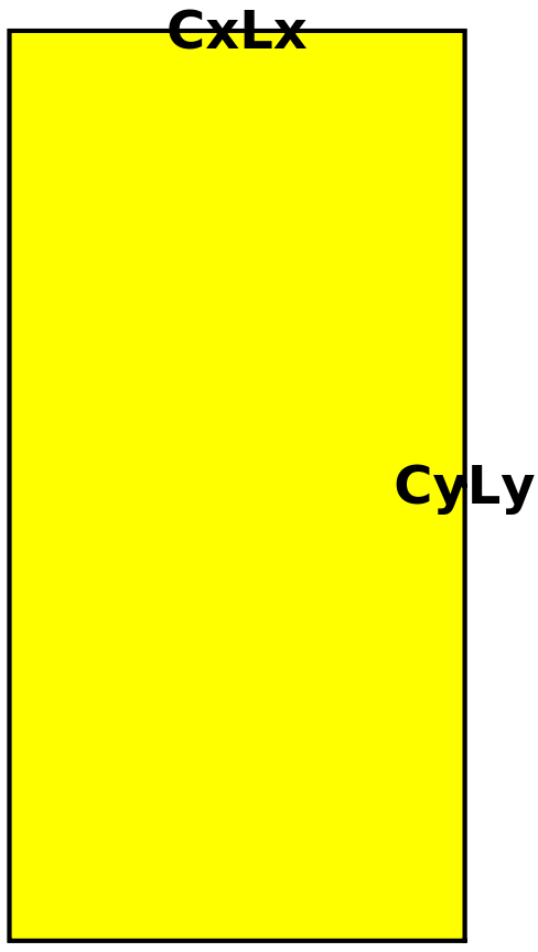
Note: Unlike Staddon and colleagues (published in Soft Matter 2023) using periodic boundary condition, we consider open boundary such that when the cell relaxes, it does not constrained by box size (CxLx * CyLy).
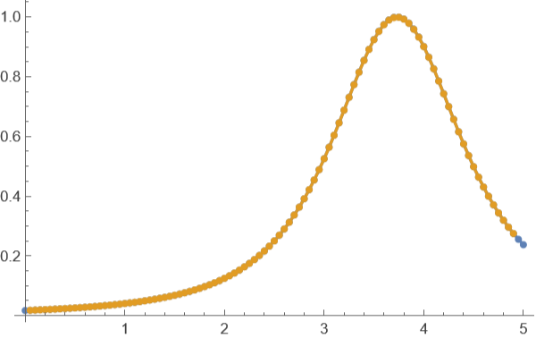
We now define a function to calculate discrete curvature along our deformed structure. This function is essential for evaluating mechanical responses of our cellular system. This measurement is crucial for observing phase transition point (when mechanical stress vanishes or property changes).
Discrete Curvature Calculation This formula calculates the curvature at point i using three consecutive points on a 2 D curve . Input : t1 - array of points representing the curve, where t1[[i]] contains {x, y} coordinates Method : Uses the circumscribed circle approach where curvature = 4 A/(abc) where A is the triangle area formed by three consecutive points and a, b, c are the lengths of the triangle sides . The numerator calculates 2 A using cross product The denominator is the product of the three side lengths Higher curvature values indicate sharper bends in the curve
CurvtureFunc[t1_,i_]:=2*Abs[((t1[[i-1,1]]-t1[[i,1]])*(t1[[i+1,2]]-t1[[i,2]])-(t1[[i-1,2]]-t1[[i,2]])*(t1[[i+1,1]]-t1[[i,1]]))]/(Sqrt[(t1[[i-1,1]]-t1[[i,1]])^2+(t1[[i-1,2]]-t1[[i,2]])^2]*Sqrt[(t1[[i+1,1]]-t1[[i,1]])^2+(t1[[i+1,2]]-t1[[i,2]])^2]*Sqrt[(t1[[i-1,1]]-t1[[i+1,1]])^2+(t1[[i-1,2]]-t1[[i+1,2]])^2]);
Analysis of Shape Index and Curvature Relationship We examine the analytical solution for mechanical stability using the function : f(p0) = 1/2 (2 + - p0)^2 where p0 is the dimensionless shape index. The code: 1. Generates data points for the function across p0 values from 0 to 52. Compares theoretical curvature (using ArcCurvature) with discrete curvature 3. Plots both curves to verify our discrete curvature implementation
3
t1=Table[{p0,1/2(2+Sqrt[3]-p0)^2},{p0,0,5,0.05}];Curv=ArcCurvature[1/2(2+Sqrt[3]-p0)^2,p0];ListLinePlot[{Table[{p0,Curv},{p0,0,5,0.05}],Table[{t1[[i,1]],CurvtureFunc[t1,i]},{i,2,99,1}]},Mesh->All,PlotRange->All]
Out[]=
Methods: deformation protocol and determining elastic moduli
Methods: deformation protocol and determining elastic moduli
Graphical explanation of Fig. 7
Graphical explanation of Fig. 7
Example. Measuring Young’s modulus of the hexagonal cells
To understand how our cellular material responds to deformation, we first examine hexagonal cells as the simplest two-dimensional case. We measure Young’s modulus, which quantifies how the material resists stretching, by applying small strains and analyzing the resulting energy changes. In our approach, we start with a reference hexagonal cell having unit area and systematically deform it along one axis while maintaining a fixed shape index. The curvature of the energy landscape near equilibrium directly relates to the Young’s modulus - a steeper curvature indicates a stiffer material. By repeating this analysis across different shape indices, we can identify where the material transitions from a rigid to a floppy state.
To understand how our cellular material responds to deformation, we first examine hexagonal cells as the simplest two-dimensional case. We measure Young’s modulus, which quantifies how the material resists stretching, by applying small strains and analyzing the resulting energy changes. In our approach, we start with a reference hexagonal cell having unit area and systematically deform it along one axis while maintaining a fixed shape index. The curvature of the energy landscape near equilibrium directly relates to the Young’s modulus - a steeper curvature indicates a stiffer material. By repeating this analysis across different shape indices, we can identify where the material transitions from a rigid to a floppy state.
In[]:=
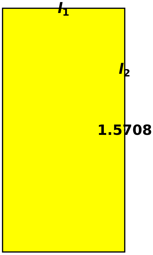
(*First,wewillparameterizehexagonusingtwosidelength(l1,l2)*)polhex[l1_,l2_,x_,y_,θ_]:={{(l1/2-l2*Cos[θ])x,0},{l1x/2,l2*y*Sin[θ]},{-l1x/2,l2*y*Sin[θ]},{(-l1/2+l2*Cos[θ])x,0},{-l1x/2,-l2*y*Sin[θ]},{l1x/2,-l2*y*Sin[θ]}};ManipulateGraphics[{EdgeForm[Thick],Yellow,Polygon[polhex[l1,l2,1,1,θ]],Black,Text[Style[,Large,Bold],({(l1/2-l2*Cos[θ]),0}+{l1/2,l2*Sin[θ]})/2],Text[Style[,Large,Bold],({0,l2*Sin[θ]})],Text[Style[,Large,Bold],({(l1/2-l2*Cos[θ]),0})]}],{θ,π/2,π},l1,,1,l2,,1,SaveDefinitions->True
l
2
l
1
θ
2
3/4
3
2
3/4
3
Out[]=


Energy Function for Cellular Mechanics We model cellular mechanics using two key contributions to the energy in a vertex model framework.
The first contribution comes from area elasticity, where (A - A0)^2 represents resistance to area changes from the equilibrium area A0 = 1. The second contribution comes from perimeter elasticity, where (P - P0)^2 represents the actomyosin cortex’ s resistance to perimeter changes. Here, P0 is the preferred perimeter, also known as the shape index. The model consists of three main functions : Ahex calculates the area of a hexagonal cell Phex calculates the perimeter of a hexagonal cell Ehex combines both contributions into the total energy with spring constant kr
The model takes several parameters :
l1, l2 define cell dimensions as two distinct side lengths .
x, y are deformation parameters representing affine deformation along respective axes .
θ represents the angular parameter (between l1 and l2) .
kr determines the relative strength of the perimeter spring .
p0 is the target perimeter at unit area, equivalent to the shape index .
In[]:=
Ahex[l1_,l2_,x_,y_,θ_]:=2l2xy(l1-l2Cos[θ])Sin[θ];Phex[l1_,l2_,x_,y_,θ_]:=2l1x+4l2Sqrt[x^2Cos[θ]^2+y^2Sin[θ]^2];Ehex[l1_,l2_,x_,y_,θ_,kr_,p0_]:=1/2((Ahex[l1,l2,x,y,θ]-1)^2+kr(Phex[l1,l2,x,y,θ]-p0)^2)
Finding equilibrium cell dimensions We solve for the side lengths l1, l2 that satisfy two conditions: 1. The cell has unit area (A = 1)2. The perimeter matches a regular hexagon with area 1 These equations ensure our reference cell has the correct geometry before we apply deformations.
p=
(8
3
)Solve[2l1+4l2Sqrt[1^2Cos[2π/3]^2+1^2Sin[2π/3]^2]-Sqrt[8Sqrt[3]]==0&&2l2(l1-l2Cos[2π/3])Sin[2π/3]-1==0,{l1,l2}]
Out[]=
l1,l2
2
3/4
3
2
3/4
3
Solution - regular hexagon with unit area 1
In[]:=
l10hex=;l20hex=;
2
3/4
3
2
3/4
3
Affine deformation of the box
In[]:=
ManipulateGraphics[{EdgeForm[Thick],White,Polygon[{{(l10hex/2-l20hex*Cos[θ])x,-l20hex*y*Sin[θ]},{(l10hex/2-l20hex*Cos[θ])x,l20hex*y*Sin[θ]},{-(l10hex/2-l20hex*Cos[θ])x,l20hex*y*Sin[θ]},{-(l10hex/2-l20hex*Cos[θ])x,-l20hex*y*Sin[θ]}}],Yellow,Polygon[polhex[l10hex,l20hex,x,y,θ]],Black,Text[Style["CyLy",Large,Bold],{(l10hex/2x-l20hex*Cos[θ]y),0}],Text[Style["CxLx",Large,Bold],({0,l20hex*Sin[θ]y})]}],{θ,π/2,π},x,,1,y,,1,SaveDefinitions->True
2
3/4
3
2
3/4
3
Out[]=
B. Moduli in two dimensions
B. Moduli in two dimensions
Fig.8 E & Fig. 11 C: We start by computing the discrete curvature of the energy function. To be precise in the case of the Young’s modulus, for example, we measure es by varying Cx over (1 − 0.0005, 1 + 0.0005). We then calculate the discrete curvature K for every data point. (p0=0~5)
Calculate Young's Modulus Through Energy Curvature Analysis Process:
1. Vary strain (deltaw) from-0.0005 to 0.0005 around x=1
2. For each p0 value (0 to 5),calculate:-Energy at different strains-Curvature of energy-strain relationship-Local slope at x=1 (represents Young's modulus at Cx=1)
1. Vary strain (deltaw) from-0.0005 to 0.0005 around x=1
2. For each p0 value (0 to 5),calculate:-Energy at different strains-Curvature of energy-strain relationship-Local slope at x=1 (represents Young's modulus at Cx=1)
Parameters:
n=50 (number of p0 intervals)
kr=0.1 (fixed perimeter spring constant)
θ=2π/3 (fixed angle)
l10hex,l20hex (equilibrium cell dimensions) Output:p0tableno stores shape index and corresponding Young's modulus values
n=50 (number of p0 intervals)
kr=0.1 (fixed perimeter spring constant)
θ=2π/3 (fixed angle)
l10hex,l20hex (equilibrium cell dimensions) Output:p0tableno stores shape index and corresponding Young's modulus values
Performance Note
Computational considerations:
1. Each calculation run requires several minutes to complete
2. The Mathematica kernel may need to reset due to dynamic chart updates
when you click the chart during computation
Please be patient during calculations
Computational considerations:
1. Each calculation run requires several minutes to complete
2. The Mathematica kernel may need to reset due to dynamic chart updates
when you click the chart during computation
Please be patient during calculations
Note on Mechanical Property and Phase Transition The Young’ s modulus analysis reveals a critical physical transition : The material undergoes a rigidity transition at shape index p0 = 3.72 where Young’ s modulus vanishes, marking the boundary between rigid and floppy states
Example. Measuring Young’s modulus of the octagonal cells
While octagonal cells by themselves cannot perfectly tile a two-dimensional space, we analyze them as an important intermediate case. Their geometry shares key features with truncated octahedra, which are the three-dimensional structures at the center of our study. Although octagonal cells leave gaps when arranged in 2D, examining their mechanical properties provides valuable insights that help us bridge our understanding between hexagonal cells in 2D and truncated octahedra in 3D. Using the same approach as with hexagonal cells, we measure Young’s modulus by analyzing the energy landscape under small deformations while maintaining a fixed shape index.
While octagonal cells by themselves cannot perfectly tile a two-dimensional space, we analyze them as an important intermediate case. Their geometry shares key features with truncated octahedra, which are the three-dimensional structures at the center of our study. Although octagonal cells leave gaps when arranged in 2D, examining their mechanical properties provides valuable insights that help us bridge our understanding between hexagonal cells in 2D and truncated octahedra in 3D. Using the same approach as with hexagonal cells, we measure Young’s modulus by analyzing the energy landscape under small deformations while maintaining a fixed shape index.
First, we will parameterize octagon using two side length (l1, l2)
Energy Function for Cellular Mechanics
Fig. 14 Octagonal cell parametrization
In the example, we will adopt a different parametrization approach for the octagonal cell, drawing inspiration from Staddon et al.’s work. Instead of using conventional vertex coordinates, we express the octagon’s geometry using height (h) and width (w) parameters. Through this approach, we can see new shape landscape potentially affects the moduli.
Note: This analysis is limited to shape indices (p0) ranging from 0 to 4.8, as the system becomes trapped in extreme angular configurations at p0 values above 4.8 (due to shape change), preventing meaningful energy minimization.
Fig. 16 Young’s modulus as a function of p0 for the reparameterized octagonal model and for two different relaxed cases.
C. Moduli in three dimensions
C. Moduli in three dimensions
Truncated Octahedron
Extract Face Information for Truncated Octahedron Use PolyhedronData function to obtain the face indices that define the connectivity of vertices in a truncated octahedron . This information is essential for constructing and visualizing the polyhedron
Define cell energy function
Finding the Reference Cell Dimensions We solve for the side length of a regular truncated octahedron that : 1. Has unit volume (V = 1) 2. Maintains the standard geometric ratios of a regular truncated octahedron This establishes our reference cell before applying deformations
Fig. 18 C Mechanical response for the truncated octahedron model.
Parametrization of truncated octahedron using h,h2,w (please check octagon parametrization for details, as truncated octahedron can look like overlapping octagonal arrays at z=0)
Fig. 20 (b) (c) Mechanical response for the reparameterized truncated octahedron model as a function of the dimensionless shape index.
Note on Relaxation Behavior Mechanical response (Young’ s modulus) shows interesting behavior around p0 = 5.5 :
1. When relaxing using only y, θ parameters : The response drops and then increases due to shape changes and insufficient relaxation
2. When relaxing four parameters : The system becomes floppy
1. When relaxing using only y, θ parameters : The response drops and then increases due to shape changes and insufficient relaxation
2. When relaxing four parameters : The system becomes floppy
Example. Additional analysis of energy function
Appendix C: detailed analysis for compatible-incompatible transition
Appendix C: detailed analysis for compatible-incompatible transition
B. Compatible state in three dimensions
B. Compatible state in three dimensions
Setting Reference Cell Dimensions for Truncated Octahedron We solve two simultaneous equations :
1. Surface area equation : toArea[l1, l2, l1, 1, 1, θ, l3] = s0
2. Volume constraint : toVolume[l1, l2, l1, 1, 1, θ, l3] = 1
These equations ensure our reference cell has : -Desired surface area (s0) - Unit volume - Proper geometric relationships between edges
1. Surface area equation : toArea[l1, l2, l1, 1, 1, θ, l3] = s0
2. Volume constraint : toVolume[l1, l2, l1, 1, 1, θ, l3] = 1
These equations ensure our reference cell has : -Desired surface area (s0) - Unit volume - Proper geometric relationships between edges
Fig. A2 (a): Area function mapping
Using 3D contour plot, we will explore energy landscape changes along the surface area s. When s is at its minimum value based on the target, there exists only one possible shape that satisfies this minimum condition. However, as s0 increases s will also increases, multiple possible shapes emerge along the contour, each satisfying the target surface area condition.
Note: These plots help visualize how the available shape configurations expand as we increase the target surface area beyond its minimum value.
For example, we can fix l1 and find solutions angle θ at s=5.5 while varying l2. Then we can see different shapes can satisfy minimum criteria. (Approximated solutions)
Visualization of Truncated Octahedron Shape Evolution Creates an interactive visualization showing how the truncated octahedron’s shape changes across different solutions that satisfy s=5.5
Parameters:
- Fixed: l1 = l103d (reference length)
- Varying: l2 = 0.5+0.01*i
- θ = solutions from NSolve (AngleAtS05p5Sol1/AngleAtS05p5Sol2)
- l3 1/(2 (l1-l2 Cos[θ]) (l1+l2 Sin[θ])) calculated to maintain geometric constraints. Uses Manipulate for interactive exploration of different configurations.
First Solution.
Squeezing in z direction induces deformation in y
Squeezing in z direction induces deformation in y
Last Solution.
Squeezing in z direction induces deformation in x
Squeezing in z direction induces deformation in x
CITE THIS NOTEBOOK
CITE THIS NOTEBOOK
Mean-field elastic moduli of a three-dimensional, cell-based vertex model
by Kyung Eun Kim, Tao Zhang & J M Schwarz
Wolfram Community, STAFF PICKS, November 29, 2024
https://community.wolfram.com/groups/-/m/t/3330805
by Kyung Eun Kim, Tao Zhang & J M Schwarz
Wolfram Community, STAFF PICKS, November 29, 2024
https://community.wolfram.com/groups/-/m/t/3330805