ABSTRACT (original article): In this study, we model a spin-network in loop quantum gravity as a regular tetrahedral lattice, applying lattice physics techniques to study its structure and vertex dynamics. Using the area eigenvalue, A∝8π , we derive a lattice constant a=2.707 and construct a vertex Hamiltonian incorporating a Lennard-Jones potential, zero-point energy, and simple harmonic oscillations. A foliation approach enforces the Wheeler-DeWitt constraint via locally non-zero Hamiltonians that globally cancel. Graviton-like perturbations (treated here as spin-0 bosons) modify the vertex energy spectrum, with variational analysis suggesting twelve coherent excitations per vertex. This model frames flat spacetime as a graviton-rich lattice while enforcing a Brownian-like stochastic picture for the gravitons, and offers a basis for extension into curved quantum geometries. CITATION (original article): N. M. MacKay (2025), “A Lattice Physics Approach to Spin-Networks in Loop Quantum Gravity,” arXiv:2507.14630. https://arxiv.org/abs/2507.14630
2
l
P
l
P
Introduction
Introduction
Loop quantum gravity (LQG) is a candidate theory to quantum gravity, looking at the spacetime geometry as fundamentally quantized structures. These result to two “bookmark” equations: the energy eigenvalue A∝8π ( is the Planck length) and the Wheeler-DeWitt Equation ψ=0. We use these equations to our advantage in the paper, when we approximate a local patch of flat spacetime (a spin-network in LQG) as a lattice.
2
l
P
l
P
H
Why tetrahedra?
Why tetrahedra?
Triangulation is an essential aspect in LQG structure modeling in a 2D representation. Each point in the lattice resembles a quantum of volume, and lattice bonds the quantum of area. Weaving points with bonds resorts to forming the most fundamental polygon in geometry: a triangle. Therefore, in a 3D extension, triangular pyramids (tetrahedra) give depth to the triangulated 2D representation. Modeling a single tetrahedral lattice cell is given as follows:
In[]:=
With[{pname="TriangularPyramid"},Module[{pts,mesh},pts=PolyhedronData[pname,"VertexCoordinates"];mesh=DelaunayMesh[pts];HighlightMesh[mesh,{Style[MeshCells[mesh,0],Directive[PointSize[Large],Black]],Style[MeshCells[mesh,2],Opacity[0.1]]}]]]
Out[]=
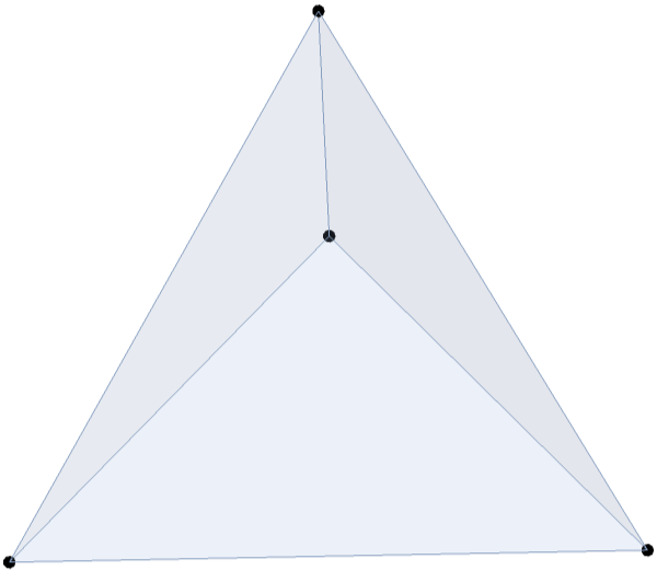
Below is the figure used in the paper.
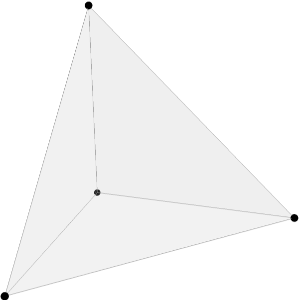
An important step in the paper is de-compacting the Wheeler-DeWitt equation with a foliation method: we slice the lattice into layers from top to bottom, isolating in each slice a non-zero, local Hamiltonian that globally annihilate. Ideally, we form an asymmetric relation between the top slice (the apex point) and the bottom slice (the base face with three points, three bonds, and a vacuous region). Out of simplicity, the work considers the single point Hamiltonian, serving as proxy to describe any lattice point in the extended lattice network. Slicing the tetrahedron to show converging slices is given as follows:
In[]:=
Module[{pts,region,slices},pts=PolyhedronData["TriangularPyramid","VertexCoordinates"];region=DelaunayMesh[pts];HighlightMesh[region,{Style[MeshCells[region,0],Directive[PointSize[Large],Black]],Style[MeshCells[region,2],Opacity[0.1]]}];slices=Table[Plot3D[zVal,{x,-1,1},{y,-1,1},RegionFunction->Function[{x,y,z},RegionMember[region][{x,y,zVal}]],PlotStyle->Directive[ColorData["AvocadoColors"][zVal],Opacity[0.4]],Mesh->None,PlotPoints->45,PlotRange->All],{zVal,-1,1.5,0.02}];Show[Graphics3D[{Opacity[0],region}],Sequence@@slices,Axes->False,Boxed->False]]
Out[]=

Below is the figure used in the paper.

Plotting the structural energy
Plotting the structural energy
A key finding in the lattice point Hamiltonian is the so-called “structural energy,” which depends on a constant quantum zero-point energy, and displacement-dependent angular momentum barriers and the Lennard-Jones potential that balances Pauli repulsion with dipole attraction. It is found that all these contributions depend on the azimuthal number l, extending the importance of angular momentum to spin-network structure. To test how l influences the structural energy, we express the energy as an argument-dependent function, and test l=1 under various displacements in terms of the “null point” σ (where the repulsion and attraction evens out):
In[]:=
U[l_,r_]:=m*c^2*l(l+1)((4.3610/Sqrt[l(l+1)])+0.4908(sigma/r)^2+1.9632((sigma/r)^{12}-(sigma/r)^6))U[1,sigma]U[1,sigma/0.8676]U[1,Infinity]
Out[]=
{7.14899m}
2
c
Out[]=
{5.94588m}
2
c
Out[]=
{6.16739m}
2
c
We’ll also test the energy as a continuous function, under linearly increasing whole values of l:
In[]:=
LogLinearPlot{U[1,x*sigma]/(mc^2),U[2,x*sigma]/(mc^2),U[3,x*sigma]/(mc^2),U[4,x*sigma]/(mc^2)},{x,0.5,50},Frame->True,FrameStyle->Directive[Black],PlotStyle->{{},Dashed,DotDashed,Dashing[0.005]},FrameLabel->"()",None,{"r/σ",None},PlotLegends->Placed[{"ℓ=1","ℓ=2","ℓ=3","ℓ=4"},{0.75,0.75}]
U
s
m
P
2
c
Out[]=
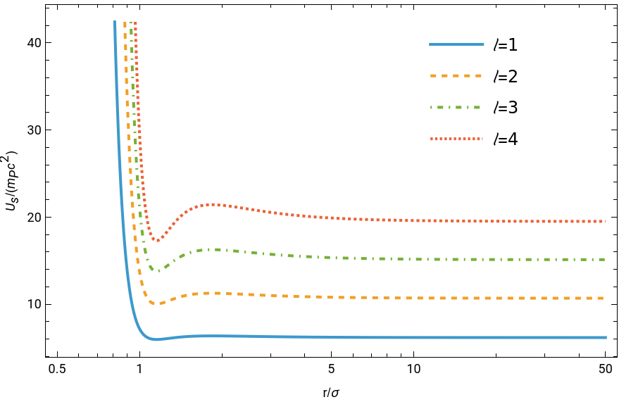
As discussed in the paper, the increase in l enhances the zero-point energy and makes the barrier well deeper with steeper walls.
A regularization calculator
A regularization calculator
One more important finding is the perturbed energy of the lattice point due to vibrations from neighboring lattice points. These vibrations are quantized as free gas gravitons (here, spin-0 gravitons), which introduce a perturbing Hamiltonian in the form of =c. With the structural energy (and the vibrational energy of the reference lattice itself) being a spectrum, imposing a variational method involved utilizing regularization techniques used to renormalize infinity calculations in QFT.
H
p
First, we have our ansatz wavefunction act on the perturbation and use it to find the perturbation’s expectation value:
Because the unperturbed energy is not operator-dependent and is a divergent spectrum, the expected value requires us to use a toy variable ξ, which refrains calculational divergences:
Understandably, this is a monstrous evaluation. Part of the regularization technique is to Taylor expand over ξ and truncate ξ⟶0. This shows polynomial orders of ξ that are driven to zero (otherwise zero without regularization), driven to infinity (the cause of the divergence), and the ξ-independent, convergent answer otherwise hidden by the divergences. The convergent answer is the physically accepted answer, which we extract by finding the zeroth-order coefficient:
Extracting the ξ-independent term, and accepting the real counterparts, we find the length scale “b”, as found in the paper.
Concluding statement
Concluding statement
This notebook offers the more technical and complicated methods and results of the paper, exploring the geometry of a spin-network in LQG and the physics of one lattice point and its perturbations. This is hopeful thinking that this can be extended into lattices that correspond to curved spacetime geometries.
CITE THIS NOTEBOOK
CITE THIS NOTEBOOK
A lattice physics approach to spin-networks in loop quantum gravity
by Noah MacKay
Wolfram Community, STAFF PICKS, August 6, 2025
https://community.wolfram.com/groups/-/m/t/3526043
by Noah MacKay
Wolfram Community, STAFF PICKS, August 6, 2025
https://community.wolfram.com/groups/-/m/t/3526043