My idea was to make some art in which we simulate drops being ejected from a drum. The animation will be much more convincing with sound. So I will also add that as well. In fact, let’s start with the sound, and then add the visuals afterwards.
Sound
Sound
A single bass drum sound:
In[]:=
Sound@SoundNote["BassDrum"]
Out[]=
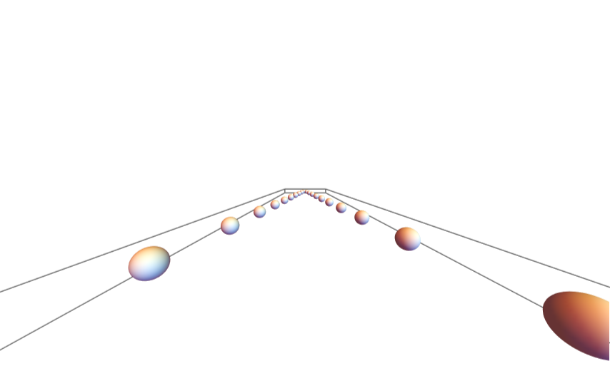
Let’s make a bunch of drums put them on two lines, alternating them left and right. Define a camera position, and two ear positions. Calculate the inverse distances (proportional to amplitude) for each ear and for each drum:
In[]:=
nmax=20;pts=Tablen,(-1)^n,0,{n,1,nmax};p={nmax+1.3,0,1};δ={0,2,0};ears={p-δ,p+δ};Graphics3D[Sphere[pts,0.2],ViewVector{p,{0,0,0}},ViewAngle90Degree,ImageSize40{16,10}]invdistances=1/Table[Norm/@Transpose[Transpose[ears]-p],{p,pts}]//Transpose;invdistances/=Max[invdistances];ListPlot[invdistances]
2n
nmax
Out[]=
Out[]=
Combine the distances, the bass drum sound, insert empty sounds, and combine everything with Δt intervals in time:
In[]:=
Δt=0.12;ϵ=0.01;beginsilence=0.2;endsilence=1;sounds=Map[SoundNote["BassDrum",ϵ,SoundVolume->#]&,invdistances,{2}];sounds//=Map[Riffle[#,SoundNote[None,Δt-ϵ]]&];sounds//=Map[Append[SoundNote[None,endsilence]]];sounds//=Map[Prepend[SoundNote[None,beginsilence]]];sounds//=Map[Append[SoundNote["BassDrum",ϵ,SoundVolume->0.00001]]];sounds//=Map[Sound];sounds//=Map[AudioData/*Mean];aud=Audio[sounds]dur=QuantityMagnitude[Duration[%],"Seconds"]Ts=Most[Accumulate[Join[{beginsilence},ConstantArray[Δt,nmax]]]];
Out[]=
Out[]=
3.50621
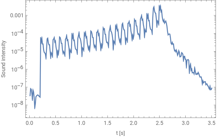
Plot the mean amplitude of the sound as a function of time:
In[]:=
blocksize=500;qm=QuantityMagnitude[Information[aud,"SampleRate"],"Samples"/"Seconds"];bmd=BlockMap[Mean,Mean[Abs[AudioData[aud]]],blocksize];bmd=Transpose[{Range[Length[bmd]],bmd}];ListLogPlot[bmdblocksize/qm,FrameTrue,JoinedTrue,FrameLabel{"t [s]","Sound intensity"}]
Out[]=
Graphics
Graphics
For each drum we need to know the velocity vector (direction) it makes as function of radius. Here for drum of unit radius:
In[]:=
ClearAll[DrumAmplitude,DrumDerivative,DrumNormal,DrumVelocity,DrumVelocity3D]DrumAmplitude[r_?NumericQ,A_?NumericQ]:=ASin[BesselJZero[0,1]]BesselJ[0,rBesselJZero[0,1]]DrumDerivative[r_?NumericQ,A_?NumericQ]:=A(-BesselJ[1,rBesselJZero[0,1]]BesselJZero[0,1]Sin[BesselJZero[0,1]])(*D[Sin[BesselJZero[0,1]]BesselJ[0,rBesselJZero[0,1]],r]*)DrumNormal[r_?NumericQ,A_?NumericQ]:=Module[{d,t,n},d=DrumDerivative[r,A];t={1,d};n={{0,-1},{1,0}}.t;Normalize[n]]DrumVelocity[r_?NumericQ,A_?NumericQ,V_?NumericQ]:=DrumNormal[r,A]DrumAmplitude[r,V]DrumVelocity3D[p:{x_,y_},A_?NumericQ,V_?NumericQ]:=Module[{r,v,v3},r=Norm[p];v=DrumVelocity[r,A,V];Append[pv[[1]],v[[2]]]]
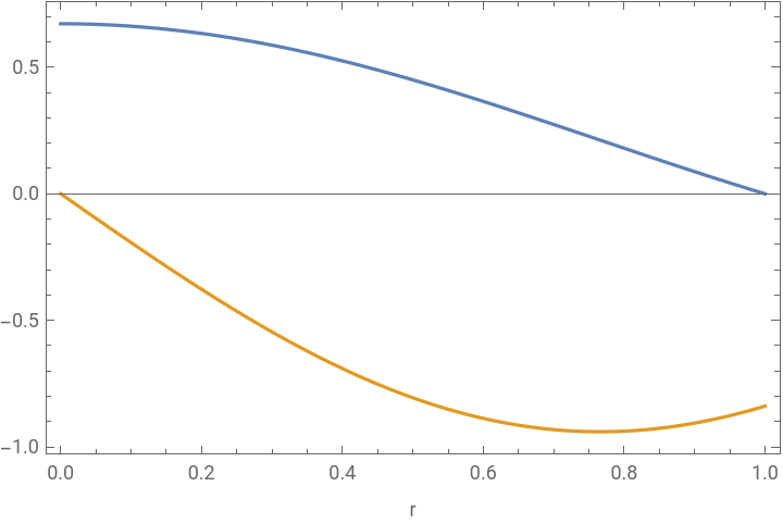
Plot the amplitude of the drum, and the derivative (used for the normal):
In[]:=
Plot[{DrumAmplitude[r,1],DrumDerivative[r,1]},{r,0,1},FrameTrue,FrameLabel{"r",None}]
Out[]=
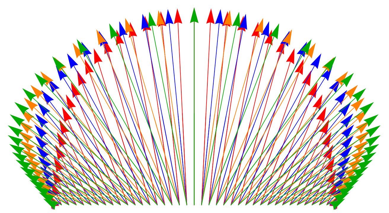
Show a couple of droplet vectors for some amplitudes for a single ‘velocity’ from a drum:
In[]:=
Table[{{Red,Blue,Orange,Darker@Green}[[i]],Table[Arrow[{{r,0},{r,0}+DrumVelocity[r,{0.5,1,1.5,2}[[i]],2]}],{r,-0.95,0.95,0.05}]},{i,4}]//Graphics
Out[]=
Test out splashing direction of a circular unit-drum:
Simple version:
Add a bit of a motion-blur:
Export the video: