In[]:=
SetDirectory[NotebookDirectory[]]
Out[]=
/Users/ecbrown/src/QTAIM.wl/QTAIM
In[]:=
Needs["QTAIM`"];(*ParallelNeeds["QTAIM`"]*)
You must compile a MathLink executable. Please see project page for details.
In[]:=
link=Install["/Users/ecbrown/src/QTAIM.wl/QTAIM/QTAIM/qtaim"];(*ParallelEvaluate[link=Install["/Users/ecbrown/src/QTAIM.wl/QTAIM/QTAIM/qtaim"]];*)
In[]:=
(*Uninstall[link];*)(*ParallelEvaluate[Uninstall[link]];*)
Wavefunction
Wavefunction
These are the workhorse functions, you need these! They are a convenient way to call the MathLink functions that compute the electron density and its various derivatives:
In[]:=
ElectronDensityDerivative[wfn_,{x_?NumericQ,y_?NumericQ,z_?NumericQ},{nx_?IntegerQ,ny_?IntegerQ,nz_?IntegerQ}]:=Module[{nmo=wfn["NumberOfOccupiedMolecularOrbitals"],np=wfn["NumberOfPrimitives"],l=wfn["l"],xp=wfn["xp"],yp=wfn["yp"],zp=wfn["zp"],a=wfn["PrimitiveExponents"],o=wfn["MolecularOrbitalOccupationNumbers"],c=Flatten[wfn["MolecularOrbitalPrimitiveCoefficients"]],link,res},res=rho1[nmo,np,x,y,z,nx,ny,nz,xp,yp,zp,l[[All,1]],l[[All,2]],l[[All,3]],a,c,o];res];
In[]:=
ElectronDensityDerivative[wfn_,xyz_?MatrixQ,deriv_?MatrixQ]:=Module[{nn=Length[xyz],nd=Length[deriv],nmo=wfn["NumberOfOccupiedMolecularOrbitals"],np=wfn["NumberOfPrimitives"],l=wfn["l"],xp=wfn["xp"],yp=wfn["yp"],zp=wfn["zp"],a=wfn["PrimitiveExponents"],o=wfn["MolecularOrbitalOccupationNumbers"],c=Flatten[wfn["MolecularOrbitalPrimitiveCoefficients"]],res},res=rhod[nn,nd,nmo,np,xyz[[All,1]],xyz[[All,2]],xyz[[All,3]],deriv[[All,1]],deriv[[All,2]],deriv[[All,3]],xp,yp,zp,l[[All,1]],l[[All,2]],l[[All,3]],a,c,o];Transpose[Partition[res,Length[xyz]]]];
Electron Density, Gradient, and Hessian:
rho[{x_?NumericQ,y_?NumericQ,z_?NumericQ}]:=ElectronDensityDerivative[w,{x,y,z},{0,0,0}];g[{x_?NumericQ,y_?NumericQ,z_?NumericQ}]:=First[ElectronDensityDerivative[w,{{x,y,z}},{{1,0,0},{0,1,0},{0,0,1}}]];grx[{x_?NumericQ,y_?NumericQ,z_?NumericQ}]:=ElectronDensityDerivative[w,{x,y,z},{1,0,0}];gry[{x_?NumericQ,y_?NumericQ,z_?NumericQ}]:=ElectronDensityDerivative[w,{x,y,z},{0,1,0}];grz[{x_?NumericQ,y_?NumericQ,z_?NumericQ}]:=ElectronDensityDerivative[w,{x,y,z},{0,0,1}];H[{x_?NumericQ,y_?NumericQ,z_?NumericQ}]:=Module[{h},h=First[ElectronDensityDerivative[w,{{x,y,z}},{{2,0,0},{1,1,0},{1,0,1},{0,2,0},{0,1,1},{0,0,2}}]];{{h[[1]],h[[2]],h[[3]]},{h[[2]],h[[4]],h[[5]]},{h[[3]],h[[5]],h[[6]]}}];
Import Existing Wavefunction from Web Server:
w=Import["https://github.com/ecbrown/QTAIM.wl/blob/master/resource/water-cas1010-ccpvdz-pyscf.wdx"];
Alternative ways to import wavefunctions: (most want WFN files I’d expect)
From a WFN File
From a WFN File
From a WFX on a HTTPS Server
From a WFX on a HTTPS Server
From PySCF
From PySCF
Nuclear Critical Points
Nuclear Critical Points
Molecular Graph
Molecular Graph
Bond Paths
Bond Paths
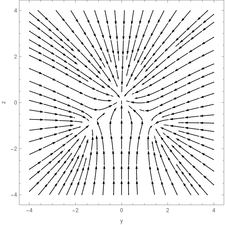
Gradient of the Electron Density
Gradient of the Electron Density
In[]:=
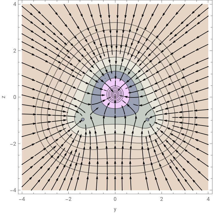
gryz[{y_?NumericQ,z_?NumericQ}]:=First[ElectronDensityDerivative[w,{{0,y,z}},{{0,1,0},{0,0,1}}]];stream=StreamPlot[gryz[{y,z}],{y,-4,4},{z,-4,4},FrameLabel{"y","z"},StreamStyle->Black,StreamColorFunctionNone]
Out[]=
In[]:=
Show[rhoPlot,stream]
Out[]=
Show[SliceContourPlot3D[rho[{x,y,z}],"CenterPlanes",{x,-2,2},{y,-2,2},{z,-2,2},AxesLabel{"x","y","z"},Contours->$QTAIMContoursPositive,PlotRange->All],graph]
In[]:=
Show[SliceVectorPlot3D[g[{x,y,z}],"CenterPlanes",{x,-2,2},{y,-2,2},{z,-2,2},AxesLabel{"x","y","z"},PlotRange->All],graph]
Plots of Atomic Basins
Plots of Atomic Basins
Miscellaneous
Miscellaneous
Classic examples from traditional QTAIM and Bader’s AIM book.
Enclosing envelope at “0.001 a.u.”
Mesh:
Solid:
Zero Laplacian Surface:
Laplacian in a plane, lone pairs are maxima front/right.
Epilogue
Epilogue