CITE THIS NOTEBOOK: PID (Proportional-integral-derivative) controller of a heater in a house by Sangdon Lee. Wolfram Community OCT 13 2022.
CITE THIS NOTEBOOK: PID (Proportional-integral-derivative) controller of a heater in a house by Sangdon Lee. Wolfram Community OCT 13 2022.
Introduction
Introduction
This is an example on how to model the PID control of a heater in a house using ParametricNDSolve[] and Manipulate[] functions. Proportional-integral-derivative (PID) control is widely used in industry.
The desired temperature of a house is 100 degree in Fahrenheit and the actual temperature is 0 degree. The desired and actual values are set intentionally to analyze the impact of KP, KI, and KD which are the coefficients for the proportional, integral, and derivative terms respectively. For example, kP = 0.1 = 1/10, which is identical to “1/time to adjust”, that is, it takes 10 minutes that the actual temperature will reach 63% of the step input (normalized as the desired temperature of 100).
The desired temperature of a house is 100 degree in Fahrenheit and the actual temperature is 0 degree. The desired and actual values are set intentionally to analyze the impact of KP, KI, and KD which are the coefficients for the proportional, integral, and derivative terms respectively. For example, kP = 0.1 = 1/10, which is identical to “1/time to adjust”, that is, it takes 10 minutes that the actual temperature will reach 63% of the step input (normalized as the desired temperature of 100).
Stock and flow diagram
Stock and flow diagram
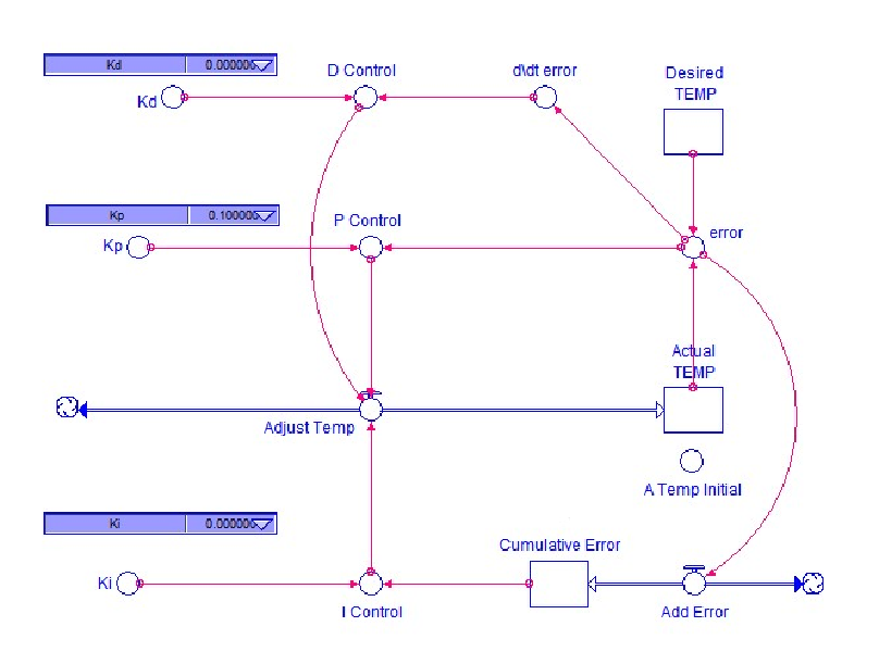
The mathematical form of PID control input, u[t], can be understood better using the stock and flow diagram below. Note that state variable, x[t], is called stock (i.e., ., rectangular box) and the derivative, "dx[t]/dt", is called flow (i.e., pipes with arrows at both ends ) . in System Dynamics. Circles are auxiliary variables for intermediate steps and they can be plotted later .
Mathematical form of PID control input
Mathematical form of PID control input
◼
u(t)=*error(t)+*error(τ)τ+*error(t)+
K
P
K
I
t
∫
0
K
d
t
◼
Proportional control
◼
Proportional control is the one that people use naturally. It tries to reduce the gap between desired temperature (desired state) and measured temperature (actual state).
◼
pControl[t]==kP*error[t]
◼
Note that any coefficient (e.g, kP=0.1) can be converted into
1
timetoadjust
◼
e.g., kP = 0.1 = 1/10 = 1/Time to adjust ==> 10 minutes to reach 63% of the step input
◼
Integral control
◼
The τ is a dummy variable.
◼
Control[t]==kI*cumulativeError[t] ,
◼
Derivative control
◼
dControl[t]==kD*(dTemp'[t]-aTemp'[t]) (* derivative control uses x'[t]. This is the key!*)
◼
Taking derivative of measure data is intrinsically unstable, e.g., measured data is jagged with noises, so in practice, filtering or smoothing is applied before taking a derivative
Modeling
Modeling
In[]:=
sol=ParametricNDSolve[{(*statevariables*)(*dTemp[t]:desiredtemperature,aTemp[t]:actualtemperature*)(*stepinputof100degreeFismodeledusingthefollowingtwothings*)(*1.dTemp'[t]==0,sothedesiredtemperatureremainsaconstant.*)(*2.dTemp[0]==100,stepinput*)dTemp'[t]==0.0,aTemp'[t]==pControl[t]+iControl[t]+dControl[t],cumulativeError'[t]==error[t],(*Auxiliaryvariablestoplotlater*)(*Auxiliaryvariablesmustbedefinedas(1)astatevariablewithnoinitialvaluedefined,and(2)followedby",".*)error[t]==(dTemp[t]-aTemp[t])(*auxiliaryvariable*),pControl[t]==kP*error[t](*proportionalcontrol,auxiliaryvariabl*),iControl[t]==kI*cumulativeError[t](*integralcontrol,auxiliaryvariabl*),dControl[t]==kD*(dTemp'[t]-aTemp'[t])(*derivativecontrolusesx'[t].Thisisthekey!*),(*initialvaluesforstatevariables*)dTemp[0]==dT0,aTemp[0]==aT0,cumulativeError[0]==0},{dTemp,aTemp,cumulativeError,error,pControl,iControl,dControl}(*dTemp,aTempandcumulativeErrorarestatevariablesbecausetheirderevativearedefined*)(*NotethateitherdTempordTemp[t]canbeusedbut"dTemp"ispreferedwaybecausedTemp'[t]ordTemp''[t]canbecomputedandplottedlater*)(*ALLauxiliaryvariablesmustbedefined:error,pControl,iControl,dControl*),{t,0,40},{dT0,aT0,kP,kI,kD}(*parameterstoadjust*)];
In[]:=
NSolve[1/timeToAdjust==0.1,timeToAdjust](*Themeaningofkp=0.1.1/timetoadjust=kp=0.1==>ittakes10minutestoreach63%ofstepinput*)
Out[]=
{{timeToAdjust10.}}
Simulate
Simulate
In[]:=
Manipulate[Row@{Plot[Evaluate[{dTemp[dT0,aT0,kP,kI,kD][t],aTemp[dT0,aT0,kP,kI,kD][t]}/.sol],{t,0,80},PlotLegendsPlaced[{"Desired Temp","Actual Temp"},Above],PlotRange{{0,40},{0,200}},ImageSize300,FrameTrue,GridLinesAutomatic],Plot[Evaluate[{error[dT0,aT0,kP,kI,kD][t],pControl[dT0,aT0,kP,kI,kD][t],iControl[dT0,aT0,kP,kI,kD][t],dControl[dT0,aT0,kP,kI,kD][t]}/.sol],{t,0,40},PlotLegendsPlaced[{"Temp. Diff.","P control","I control","D control"},Above],PlotRange{{0,40},{-100,100}},ImageSize300,FrameTrue,GridLinesAutomatic],Plot[Evaluate[{dTemp[dT0,aT0,kP,kI,kD]'[t],aTemp[dT0,aT0,kP,kI,kD]'[t]}/.sol],{t,0,40},PlotLegendsPlaced[{"d/dt dTemp","d/dt aTemp"},Above],PlotRange{{0,40},{-50,50}},ImageSize300,FrameTrue,GridLinesAutomatic]},{{dT0,100,"Desired \n Temperature"},0.0,100,10},{{aT0,0,"Measured \n Temperature"},0.0,100,10},{{kP,0.1},0.0,1.0,0.05},{{kI,0.0},0.0,1.0,0.05},{{kD,0.0},0.0,1.0,0.05},ControlPlacement->Left,SaveDefinitions->True]
Out[]=


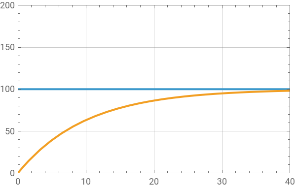


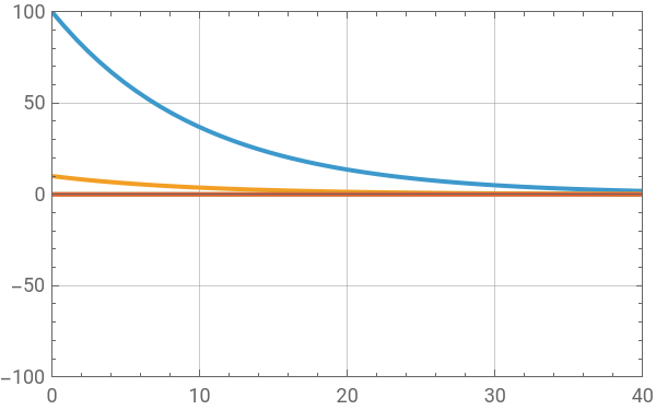
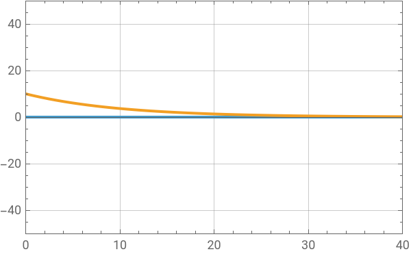
kP, kI, and kD controls
kP, kI, and kD controls