The Firing Squad Synchronization Problem is a puzzle in theoretical computer science and cellular automata. The problem characterizes a line of identical soldiers who can only see their immediate left and right neighbors. Without any global clock or knowledge, they must all reach “fire” state simultaneously after a single soldier receives a start signal. Inspired by the classical firing squad synchronization problem, this work investigates automated evolutions of synchronization rules instead of manually designed rules within a 1-D cellular automata with periodic boundary conditions. A fitness function provides an algorithm to reward configurations that maximize simultaneous firing and penalize mistakes. Through the usage of iterative random point mutation, this framework automatic discovery of local interaction rules that achieve synchronization.
Introduction
Introduction
In many natural systems, coordinated behavior must emerge despite interactions being limited to local connections. Numerous biological processes, including synchronized emergence of periodical insects, coordinated neural activity, and collective animal behavior, rely on individuals making decisions based solely on information obtained from nearby neighbors. For example, the cardiac system’s interactions between individual heart cells and neighbor cells provides an example of this phenomenon, as an impulse generated by the sinoatrial node (SA) node propagates through the cardiac tissue through electric signals, causing synchronized contractions of the heart.
This process of local consensus has been modeled previously by a system known as the Firing Squad Synchronization Problem. In 1999, Karel Culik generalized one known solution in the context of cellular automata. To avoid boundary condition, he set the problem in the context of periodic boundary conditions. Classically, traditional solutions of the FSSP hand-construct such rules for a line with two fixed, distinct endpoints. Designing such cellular automata by hand is challenging as search space grows exponentially with both the neighborhood size and the number of cell states, making exhaustive search computationally infeasible.
This experiment changes the setup in two important ways:
This process of local consensus has been modeled previously by a system known as the Firing Squad Synchronization Problem. In 1999, Karel Culik generalized one known solution in the context of cellular automata. To avoid boundary condition, he set the problem in the context of periodic boundary conditions. Classically, traditional solutions of the FSSP hand-construct such rules for a line with two fixed, distinct endpoints. Designing such cellular automata by hand is challenging as search space grows exponentially with both the neighborhood size and the number of cell states, making exhaustive search computationally infeasible.
This experiment changes the setup in two important ways:
1
.Topology. By assuming that the sites are arranged in a ring, this solution removes the boundary "walls" that classical constructions lean on, so any timing signal must synchronize using purely relative, rotationally-symmetric information
2
.Method. Rather than hand-deriving rules to achieve a perfect solution, the rules are naturally evolved via randomized local search, a stochastic method known as “Hill Climbing”.
Formally, Culik defined a cellular automaton rule with a set of 16 states including a quiescent state, a unique start state, a firing state, and additional states representing intermediate signaling pattern. For the purposes of this project, Culik’s model is simplified to an alphabet of only five states. State 0 represents the quiescent (blank) state, state 1 is the unique start state, and state 2 denotes the firing state. The remaining states, 3 and 4, act as intermediate signaling states. Beyond the firing squad synchronization problem, this framework contributes to broader studies surrounding evolutionary automation and adaptation of distributed algorithms in cellular automata.
The Firing Squad Synchronization Problem
The Firing Squad Synchronization Problem
At time (t = 0), the problem begins with a start signal given by one general. Because periodic boundary conditions are used, the first and last cells are treated as neighbors. At every subsequent time step, all soldiers update their states simultaneously according to local, uniform rules. Thus, a perfect solution would evolve a single "start" cell into a row of all "fire" cells with no firing states in any earlier row. In an ideal solution with perfect rules will achieve an optimal state where every state is firing on the final row and there are no firing states prior to this point.
To model the firing squad problem, each soldier is represented as a cell in a one-dimensional cellular automaton arranged on a ring. Each cell can occupy one of five possible states, which is represented as numeric values in our cellular automaton model.
◼
0 = Quiescent state, White
◼
1 = Start state, Blue
◼
2 = Fire state, Red
◼
3 & 4 = Two intermediate states used to transmit and process information, Yellow and Green
The goal of this algorithm is to eventually end up with a line of fully red cells, and a graph above the line with no red cells.
Basic Cellular Automaton Model
Basic Cellular Automaton Model
Search Space Calculations
Search Space Calculations
At every time step, each soldier updates their state based on their state and the states of their immediate neighbors (left, self, right). As the start state is only used once in order to begin the simulation, it will never be a value of a rule. Let S be the set of values that can appear as input. A radius-1 cellular automaton considers the left, center, and right cell; thus, the neighborhood space is =125possibleneighborhoods. A rule therefore consists of assigning one output state to each of these 125 configurations. Since a rule can never recreate the starting state, outputs are restricted to . Thus, the total number of deterministic transition rules is:
3
5
N{0,1,2,3,4}
125
4
75
10
The enormous size of this rule space makes enumeration unrealistic. Instead of using brute force to exhaustively test all possible values for every rule, we can use hill climbing to explore the space efficiently by making small random modifications and keeping beneficial changes.
Setting up Initial Rules and CA
Setting up Initial Rules and CA
Given a width w, the initial ring configuration is all-quiescent except a single excited cell (state 1) in the middle. Each subsequent row is generated by applying the current rule table to every 3-cell window, wrapping at the boundary. Each ArrayPlot is a space-time diagram, where column = soldier position, row = time step. The algorithm begins with a randomly generated list of distinct rule key to value associations. Additionally, a function is needed to create a cellular automata matrix using a list of rule associations, a set width, and a certain number of rows. Then, a function is created to generate an array plot of the result.
ruleCombinations returns a random rule with a state set of {0, ..., k - 1} with the following restrictions, no neighborhood maps to 1 which is a special start state and {0, 0, 0} always maps to 0
In[]:=
ruleCombinations[numStates_]:=Rest[Tuples[Range[0,numStates-1],{3}]]
ruleValues returns a random integer from {0, ..., k - 1} , not including 1, which is the start firing cell
In[]:=
ruleValues[numStates_]:=RandomChoice[DeleteCases[Range[0,numStates-1],1]]
createRules generates a list of rule associations pointing to random values {1, 2, ... k} for states k
In[]:=
createRules[numStates_]:=Append[Association[Table[i->ruleValues[numStates],{i,ruleCombinations[numStates]}]],{0,0,0}->0]
createStartRows creates an array of starting row states
In[]:=
createStartRow[width_]:=Flatten[{Table[0,Floor[width/2]],1,Table[0,width-Floor[width/2]-1]}]
createCellularAutomata creates cellular automaton based on width and rules
In[]:=
createCellularAutomata[rules_,width_,steps_]:=CellularAutomaton[{Lookup[rules,Key[#],0]&,{},1},createStartRow[width],{steps}];
generateGraph generates an array plot of cellular automata matrix
In[]:=
generateGraph[caMatrix_]:=ArrayPlot[caMatrix,ColorRules->{1->Blue,2->Red,3-> Green,4-> Yellow}]
Using Fitness to Score a Run
Using Fitness to Score a Run
To quantify the success of a particular set of rules, a “Fitness” function is defined to evaluate after every iteration. Based on this “Fitness” function, we can implement a greedy algorithm, accepting mutations based on their effect on the overall “Fitness” function. We will separately count graphMistakes (number of misfires before the ‘final’ row), and finalLineMistakes (number of cells that did not fire in the ‘final’ row). We can define our “Fitness” function, , using the following equation, where and represent tunable coefficients:
F
a
b
F
To calculate a graphMistakes value, we first compute a line fitness penalty for every row before the maximum-fire row. As lines get further from the final line, their respective weights increase by a factor of . This penalizes early fires more heavily the further they occur from the eventual “best” row. At line n, lineFitness can be calculated:
2
n
lineFitness
n
2
(rowsfromfinalrow)
A graphMistakes value can be produced by totaling the value of all line fitness.
countFires creates a matrix with number of fires per each row r ({1,2,3,..r})
In[]:=
ClearAll[countFires];countFires[caMatrix_]:=Count[#,2]&/@caMatrix
maxFireRow Example
maxFireRow Example
In the two graphs below, the specific row representing the peak fire count is highlighted. For visual clarity, the charts use a grayscale color scheme. Once the max row is reached, the algorithm stops calculating fitness. This highlighted row serves as the boundary for the fitness scoring algorithm: it defines the point upon which the fitness function evaluates performance, and it marks the exact threshold where all fitness calculations terminate.
Generate examples of incomplete solution vs complete solution
In[]:=
Out[]=
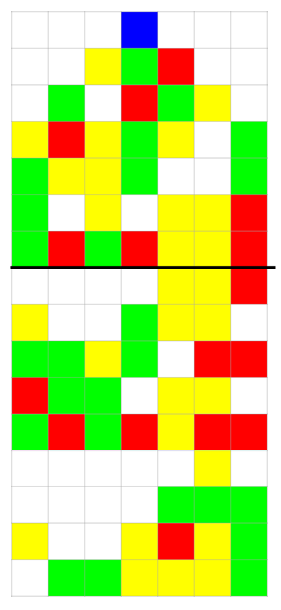
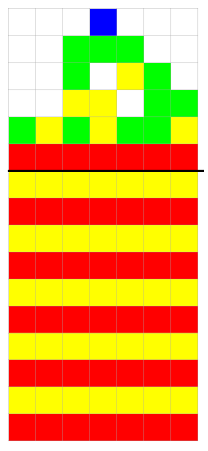
maxFireRow returns the ‘final’ row (steps) representing the number of time steps we will analyze, by determining the row consisting of the highest number of fires. In an ideal run, this row index should exclusively consist of fires.
In[]:=
ClearAll[maxFireRow];maxFireRow[countFiresList_]:=Position[countFiresList,Max[countFiresList]][[1,1]]
lineFitness returns the fitness of each line
In[]:=
lineFitness[countFiresList_,line_,finalRow_]:=(finalRow-line)^2*countFiresList[[line]]
graphMistakes returns the sum of the fitness of each line to determine the total fitness of the graph, excluding the ‘final’ row
In[]:=
graphMistakes[countFiresList_,finalRow_]:=Sum[lineFitness[countFiresList,line,finalRow],{line,1,finalRow-1}]
finalMistakes returns the number of mistakes in the final row
In[]:=
finalMistakes[width_,firesList_,finalRow_]:=width-firesList[[finalRow]]
In[]:=
falsePositiveWeight=1;falseNegativeWeight=10;
fitness returns the fitness of a given matrix by calculating finalList and finalRow
In[]:=
fitness[caMatrix_,width_]:=Module[{firesList,finalRow},firesList=countFires[caMatrix];finalRow=maxFireRow[firesList];-(falsePositiveWeight*graphMistakes[firesList,finalRow])-falseNegativeWeight*falseNegativeWeight[width,firesList,finalRow]]
Random Search Procedure and Mutation
Random Search Procedure and Mutation
Random mutations can be made on rules by adjusting the values {0, 2, 3, 4 ..., k} for states k at various random keys. A random index can be chosen in the rules list to alter, while storing both mutated rules and current rules. In case the mutation decreases the fitness, the rules list is reverted back to its original state the mutation is disregarded. Thus, it can be ensured that fitness levels never decrease, but instead either stay stagnant or increase.
findRandomKey returns value at randomKey after switching to a RandomChoice {0,2,3,4, ..., k}. 1 is not included, because for all possible algorithms, there will always be a fixed number of starting machines
In[]:=
findRandomKey[rules_]:=Module[{randomKey},randomKey=RandomChoice[DeleteCases[Keys[rules],{0,0,0}]]]
randomMutation returns rules with random values at random keys
In[]:=
randomMutation[rules_,states_]:=Module[{currentKey,currentVal,mutationChoices,newRules},currentKey=findRandomKey[rules];currentVal=rules[currentKey];mutationChoices=DeleteCases[DeleteCases[Range[0,states-1],1],currentVal];newRules=rules;newRules[currentKey]=RandomChoice[mutationChoices];{newRules,rules}]
Hill Climbing Algorithm
Hill Climbing Algorithm
Hill climbing is defined as a meta-heuristic optimization technique used commonly in artificial intelligence. It utilizes a greedy algorithm by iteratively making incremental changes to complex systems, making choices based on immediate use. FSSP is inherently based on small changes that ripple and grow in magnitude, thus, simplicity is important in order to solve the problem. Here is an example of a signal propagating through the line provides a step-by-step playback of the cellular automaton by isolating and rendering one row at a time:
Example Soldier Visualization
Example Soldier Visualization
matrixSolution stores pre-generated solution of the FSSP with width 8
Hill Climbing Code
Hill Climbing Code
Now that both the Fitness function and the RandomMutations function are defined, a hill climb algorithm can be built such that if the mutation increases fitness levels, it is kept, while if it decreases fitness levels, it is deleted. This allows different signals within rows to either be filtered, which can prevent a wandering fitness level and ensures a constantly growing or stagnant fitness level.
continueMutations returns current rules if mutated fitness is less than current fitness, else return mutated rules
runWidth generates starting rules and matrix, then continue mutations until synchronization is reached. then continueMutations runs while fitness < 0
Another aspect of the hill climbing algorithm I considered was mandating an increasing fitness level instead of allowing a stagnant one. Although this approach could increase run times, it proves to be incredibly risky in cases where a fitness level reaches the highest point in its immediate vicinity, it stops moving and ultimately becomes trapped. Because hill climbing only focuses on the immediate fitness state and its closest neighbors, in a scenario where fitness levels get stuck on a “local maxima” or “false peak”, it becomes impossible for the algorithm to escape.
Animation
Animation
To visualize the process of cell synchronization, an animation can be used to display the cellular automaton state after each accepted mutation. At each iteration, a new mutation is generated and evaluated using the fitness function. The animation begins with a poorly synchronized system with a fitness value of -60. As successful mutations are discovered, the fitness gradually improves:
runWidthHistory stores iteration, best fitness, and matrix in variable history
animationGraph creates interactive graph for matrix width 8, states 5, and steps 10
Analysis
Analysis
Using the created matrix and algorithm, analysis can be used to understand cellular automata patterns and behaviors. This section analyzes how iteration length variability, fitness level stagnation, final row instability, and rule distribution affect overall speed, behavior, and outputs of the algorithm.
Convergence Time Variability
Convergence Time Variability
To evaluate the robustness of the evolutionary algorithm, 60 independent trials were performed to model the distribution of convergence times. Each point represented the number of iterations required for the cellular automaton to reach the optimal fitness value of zero. Crucially, the algorithm reached optimal fitness for 100% of test runs, suggesting reliability in smaller widths. However, although each run eventually reached the optimal solution, but the number of iterations required varied considerably. Throughout plateaus, the 100% completion rates indicate that this algorithm must be adaptable to inevitably break out of a cycle or trap.
maxIter returns maximum iteration count
meanIter returns mean of all iteration counts
stdIter returns standard deviation of iteration counts
maxIndex returns the position of max iteration in iterList
trials creates graph ‘trials’, blue points representing # of iterations at each trial, red line representing the mean iterations number
The algorithm required an average of 8,570.43 iterations to converge, with a maximum of 50,928 iterations. The standard deviation was 11,203 iterations, showing considerable variation in convergence time between runs. The median was considerably lower than the average convergence time; it can be assumed that this disparity is caused by a small number of exceptionally long runs increasing the average, resulting in a right-skewed distribution. This skew can likely be attributed to plateaus or deceptive local optima. In a small percentage of trials, these configurations can cause trapped cycles of mutations that require more iterations to break. The exceptionally large standard deviation creates a distribution where variation cannot be interpreted via traditional symmetric bell-curve assumptions.
To quantify the asymmetry of the convergence times, the sample skewness coefficient (S) can be calculated.
Find skewness of iteration list
In statistical analysis, a skewness value of 0 indicates perfect symmetry, while any value exceeding 1.0 denotes a highly skewed distribution. Thus, a skewness result of 2.2 reveals an extreme right-shifted distribution, likely from significant high-iteration outliers. This idea can be plotted on a whisker graph, where outliers are accounted for during analysis. A box whisker graph below can be created to represent the asymmetry. The yellow container spans the interquartile range, the white dividing line pinpoints the median = 3,761, and the detached red circles isolate the extreme statistical outliers lounging above the 30,000-iteration threshold.
whiskerChart creates whisker chart with outliers isolated
Fitness Levels
Fitness Levels
The hill climbing algorithm must drift around until hitting a “breakthrough” or critical rule to move on to another fitness level, which can cause sharp vertical jumps in fitness. To isolate and evaluate the structural impact of each evolutionary breakthrough, a graph of each the absolute value of fitness per increasing jump can show asymptotic decay of intervals. As each iteration continues, the jump size drops rapidly from over 160 down to under 50 within the first five major breakthroughs. The vertical jumps between plateaus indicate instances where a critical rule mutation successfully increases fitness levels, breaking the cycle of the plateau.
When the absolute error curve is mapped onto a semi-logarithmic scale, the graph appears to be a linear trend. This demonstrates how the evolutionary framework minimizes global synchronization errors at an exponential rate.
Final Row Instability
Final Row Instability
Final row determines the number of elements in graphMistakes, which can decrease total weightings, which would otherwise increase exponentially per each row. Additionally, when the final row index continuously changes or overly large, its predictive accuracy degrades. Final-row instability can trigger faulty rule-making across a wide range of varying rows, which can lead to more unnecessary mutations, further increasing iterations and run time. Thus, it can be immensely helpful to have both a stable and small final row index.
stableFinalLine and unstableFinalLine initializes graph of ‘Iteration Count’ Vs. ‘Final Line’ index of two graphs with width 7
In Graph 1, it can be observed that as the iterations pass, the Final Line row stabilizes, eventually setting on 4. In contrast, in Graph 2, the Final Line row bounces between 5, 6, and 7 throughout all iterations, never fully settling on one constant value. Therefore, it can be assumed that with a lower, quickly stabilizing graph, the number of iterations used to reach a ' perfect solution' decreases.
Rules Analysis
Rules Analysis
To understand the structural characteristics of the evolved cellular automata algorithms, output distributions can be analyzed in a rule table. Given an alphabet size of k = 5 states ({0, 1, 2, 3, 4}) and a standard nearest-neighbor radius of r = 1 (neighborhood width of 3), the total number of distinct local configurations mapping to an output state is defined by:
Initialization of graphs
runWidthRules outputs rules for analysis
showRulesBarGraph creates and displays bar chart of grouped rules 10 times
The "fire" state exhibits a notable dependency on the spatial scale of the ring. At width 3, the density of state 2 is 33, at width 8, the density drops considerably to around 28.5. This is because, at a small ring width (N = 3), there is less of a need for complicated timing sequence, as signals can just jump straight to the firing state much quicker. Thus, the evolutionary pressure shifts away from preserving signaling capacity over longer time steps and towards committing to the terminal “fire” state. to achieve a perfect fitness score quicker. An expansion of the physical grid introduces complex long-range spatial dynamics, forcing the evolutionary algorithm to favor rules with wider propagation vectors.
Additionally, the remaining rule allocations display a highly uniform and symmetrical distribution, as each state except 2’s weight is ultimately the same, to be used for signal propulsion. Since this problem operates on a periodic boundary, synchronization cannot be achieved via a single localized signal. Instead, the evolutionary algorithm utilizes states 3 and 4 to establish directional information paths across the ring. This flat distribution of rules proves that a precise ratio of empty space, left-traveling information, and right-traveling information is universally required to produce an optimal outcome.
Solution Speed
Solution Speed
runSolutionTest function loops to continue mutations and outputs iteration i
Conclusion
Conclusion
To solve the Synchronized Firing Squad Problem and other complex puzzles in theoretical computer science, an automated approach can be used over a hand-crafted one. A hill-climbing genetic algorithm that evolves a radius-1, four-state cellular automaton rule against a fitness function derived from per-row firing-state counts. The search reliably penalizes and rewards different outcomes, using random single-rule mutations that are kept only under strict fitness improvement (Δ ≥ 0). It is able to drive fitness to its maximum value of 0 within a few hundred thousand iterations, stimulating the natural evolution and adaptation of organisms in an environment. However, as a hill climbing solution follows greedy behavior, choosing only acceptable moves within an iteration with little ability to calculate outcomes. Thus, future work should focus on a more strategic approach to anticipate and predict future actions within an iteration. Furthermore, while synthetic versions of this problem generally apply a single set of rules independent of cell width, these specific experiments utilized a fixed width. Preliminary explorations indicate that a rule evolved for one width can still achieve a large degree of success when scaled to higher ones. Thus, future work should also focus on signing the fitness function to evaluate a rule’s performance across multiple widths simultaneously to promote true scale-invariance.
Future Directions
Future Directions
Recent attempts to accelerate convergence involved target-repair mechanisms. So, the initial approach for this project was to reference this idea to fix specific mistakes within a graph, surgically altering a single rule in an attempt to decrease iteration lengths. This approach resulted in a phenomena known as catastrophic forgetting” across other regions of the space-time grid.” This behavior is thoroughly described by Das, Crutchfield, Mitchell, and Hanson (1995) in their foundational paper “Evolving Globally Synchronized Cellular Automata”. To implement a blend of both the hill climbing random approach and a specific mutation approach, the problem can be explicitly framed as a multi-objective optimization problem, attributing tunable weights to each system and choosing randomly between the two per iteration.
To run this version of the algorithm, add findKey function and replace findRandomKey and randomMutation
New Solution Code
findKey utilizes a targeted approach and finds the position of the first instance of a fire and returns its values
findRandomKey utilizes a hill climbing approach involving randomly selecting a rule key within the rules list
randomMutation changes a specific rule in a randomly selected way. Both the targeted and hill climbing approaches are assigned weightings to either system, and have an equal likelihood of being chosen
Another interesting idea to explore is the pivot to non-uniform cellular automata. Pioneered by Sipper, Tomassini, and Capcarrère (1997) in “Evolving Asynchronous and Scalable Non-uniform Cellular Automata”, this processes allows the organic patching of mistakes without degradation of the rest of the ring.
References
References
Culik, Karel. “Variations of the Firing Squad Problem and Applications.” Information Processing Letters, vol. 30, no. 3, Feb. 1989, pp. 152–57. DOI.org (Crossref), https://doi.org/10.1016/0020-0190(89)90134-8.
Sipper, Moshe, and Marco Tomassini. “Computation in Artificially Evolved, Non-Uniform Cellular Automata.” Theoretical Computer Science, vol. 217, no. 1, Mar. 1999, pp. 81–98. DOI.org (Crossref), https://doi.org/10.1016/S0304-3975(98)00151-0.
The Firing Squad Problem. https://cs.stanford.edu/people/eroberts/courses/soco/projects/2004-05/automata-theory/problem.html. Accessed 9 July 2026.
Wolfram, Stephen. “Why Does Biological Evolution Work? A Minimal Model for Biological Evolution and Other Adaptive Processes.” Stephen Wolfram Writings, May 2024. writings.stephenwolfram.com, https://writings.stephenwolfram.com/2024/05/why-does-biological-evolution-work-a-minimal-model-for-biological-evolution-and-other-adaptive-processes/.
Yunès, Jean-Baptiste. “An Intrinsically Non Minimal-Time Minsky-like 6-States Solution to the Firing Squad Synchronization Problem.” RAIRO - Theoretical Informatics and Applications, vol. 42, no. 1, Jan. 2008, pp. 55–68. DOI.org (Crossref), https://doi.org/10.1051/ita:2007051.
Acknowledgements
Acknowledgements
I would like to thank my mentor, Lyman Hurd, for his guidance throughout this project. This would not have been possible without his amazing ideas and support.
Additional thanks to Stephen Wolfram for suggesting this project, and to the directors of WSRP, Rory, Megan and Eryn, for their hard work organizing this opportunity for students. Finally, I’d like to thank the TA’s for their help, and to my TA Group for their encouragement.
CITE THIS NOTEBOOK
CITE THIS NOTEBOOK
Evolving consensus in cellular automata behavior
by Rachel Dai
Wolfram Community, STAFF PICKS, July 9, 2026
https://community.wolfram.com/groups/-/m/t/3754039
by Rachel Dai
Wolfram Community, STAFF PICKS, July 9, 2026
https://community.wolfram.com/groups/-/m/t/3754039