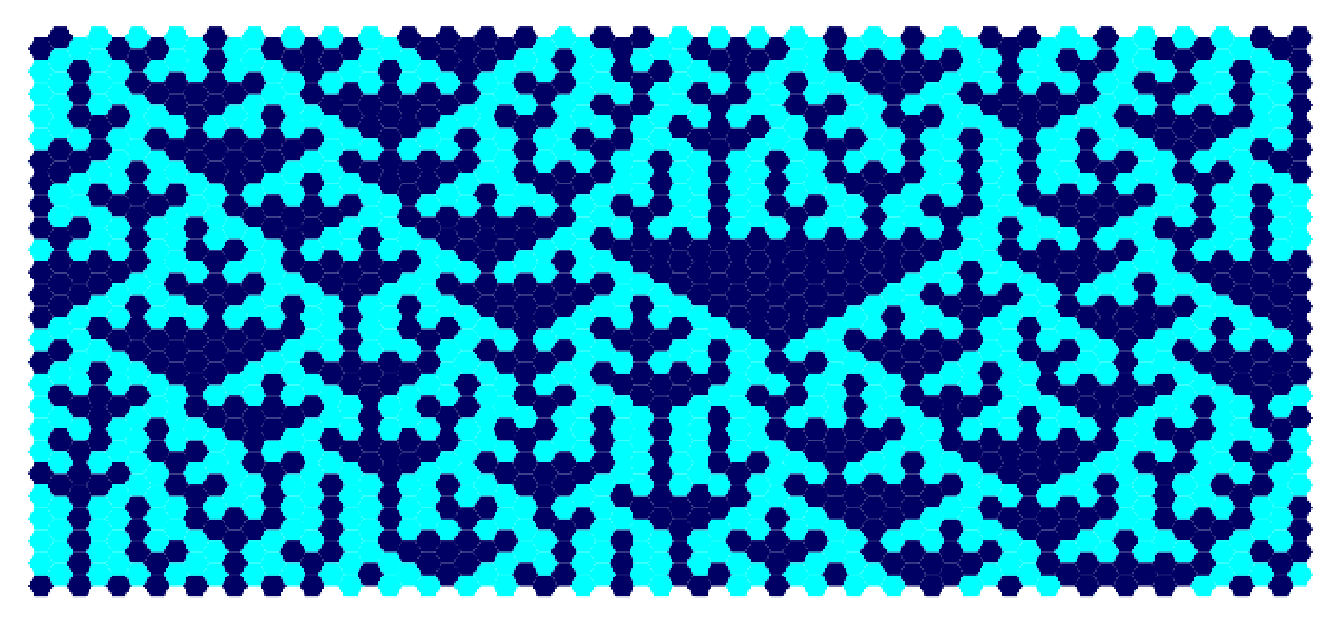
Analogs to elementary cellular automata on alternative tilings
By Chase Marangu
College of San Mateo
By Chase Marangu
College of San Mateo
Elementary Cellular Automata (ECA) are defined on a square grid. The states of the cells in each row are given by the neighboring cells one row above. This project extended the definition of an ECA to other periodic 2D tilings. For each tiling, there were multiple ways of dividing it into rows and assigning a “time” or vertical direction. After rotating the tiling to assign the vertical “time” direction, we define the rows to be the sets of polygons with centers at equivalent y-coordinates, and the neighborhoods of each cell to include cells in its Moore neighborhood with higher y-coordinates.
Original Square Tiling (3 neighbors)
Original Square Tiling (3 neighbors)
The original square tiling is the most widely used ECA grid.
Rule 30
Rule 30
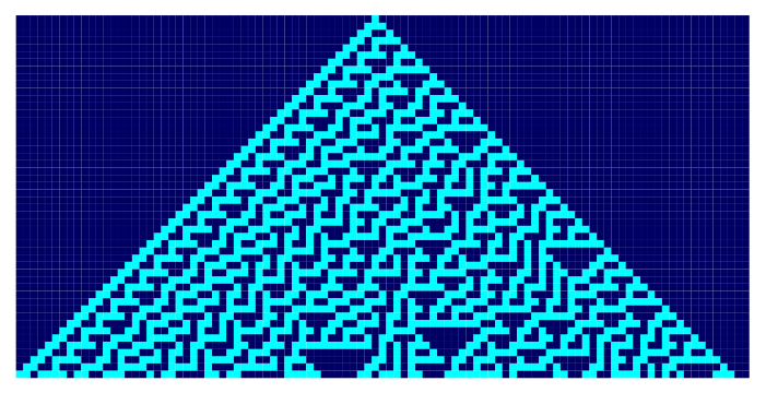
Rule 30 is one of the most well-known ECA because of the deeply complex output it generates from its relatively simple rule set.
To plot rule 30 on the original square tiling, we only need to change a few of the parameters, including the tiling type and the rule number, and (if desired) the seed type, width, and height.
This plot was generated with width 101, height 50, seed type 1 (single cell), tiling type 1, and rule number 30.
This plot was generated with width 101, height 50, seed type 1 (single cell), tiling type 1, and rule number 30.
Rule 90
Rule 90
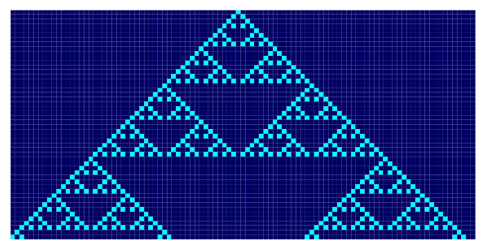
Rule 90 is another well-known ECA rule set for the square grid because of the symmetric and self-similar “nesting” structure it generates.
To plot rule 30 on the original square tiling, we only need to change a few of the parameters, including the tiling type and the rule number, and (if desired) the seed type, width, and height.
This plot was generated with width 101, height 50, seed type 1 (single cell), tiling type 1, and rule number 30.
This plot was generated with width 101, height 50, seed type 1 (single cell), tiling type 1, and rule number 30.
45° Rotated Square Tiling (3 neighbors)
45° Rotated Square Tiling (3 neighbors)
When extending the definition to other tilings, we noticed that they could be sliced into rows of polygons with centers at equal height more than one way. One interesting case was the square grid itself rotated 45°.
Rule 30
Rule 30
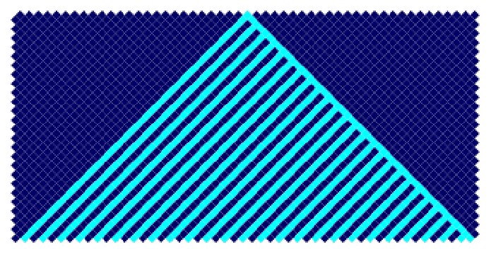
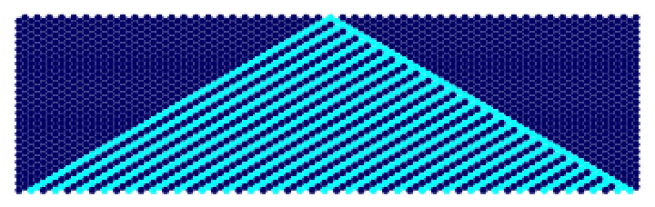
Interestingly, Rule 30 is not chaotic in the rotated square tiling. It is, however, still asymmetric under vertical reflection.
This plot was generated with width 51, height 50, seed type 1 (single cell), tiling type 1, and rule number 30.
Rule 90
Rule 90
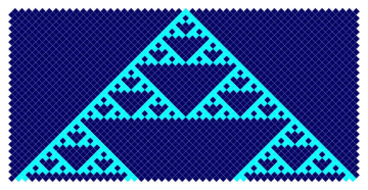
Interestingly, rule 90 on the diagonal square grid does exhibit the same “nesting” behavior as its rule 30 counterpart. This is surprising considering its rule 30 is not chaotic, but since both rules have 3 neighbors (a left, a center, and a right neighbor, in that order), the symmetry of the rule number is preserved. In this case rule 90 is symmetric in both tilings and avoids overcrowding in both tilings, leading to the mysterious fractal structure.
This plot was generated with width 51, height 50, seed type 1 (single cell), tiling type 1, and rule number 90.
Hexagon Tiling (Some Edges Horizontal, 3 neighbors)
Hexagon Tiling (Some Edges Horizontal, 3 neighbors)
If the hexagon tiling is rotated 30° so that two edges from each hexagon are horizontal, then there is a different row ordering and neighbor assignment (because of the different y-coordinates of the cells’s centers).
Comparison to 45° Rotated Square Tiling
Comparison to 45° Rotated Square Tiling
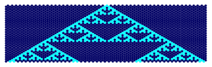
Since we defined the rows to be cells with centers identical y-coordinates and the neighbors of each cell to be the the cells in its Moore neighborhood which are also in higher rows, the hexagon tiling with 3 neighbors has identical rules and behavior to the 45° rotated square grid. This is because on both tilings, each cell has exactly 3 neighbors, 2 in the row directly above it and one two rows above it.
Other neighborhoods for both rotated square tiling and hexagon tiling (with edges horizontal) could be defined, but we decided that row assignment based on center height and neighbor assignment based on Moore neighborhood and cell y-coordinate was the best generalization of the original square tiling ECA.
Other neighborhoods for both rotated square tiling and hexagon tiling (with edges horizontal) could be defined, but we decided that row assignment based on center height and neighbor assignment based on Moore neighborhood and cell y-coordinate was the best generalization of the original square tiling ECA.
The same plot from the diagonal square grid (above) generated with width 51, height 50, seed type 1 (single cell), tiling type 1, and rule number 30, only changing tiling type to 5.
The same plot from the diagonal square grid (above) generated with width 51, height 50, seed type 1 (single cell), tiling type 1, and rule number 90, only changing tiling type to 5.
Hexagon Tiling (Some Edges Vertical, 2 neighbors)
Hexagon Tiling (Some Edges Vertical, 2 neighbors)
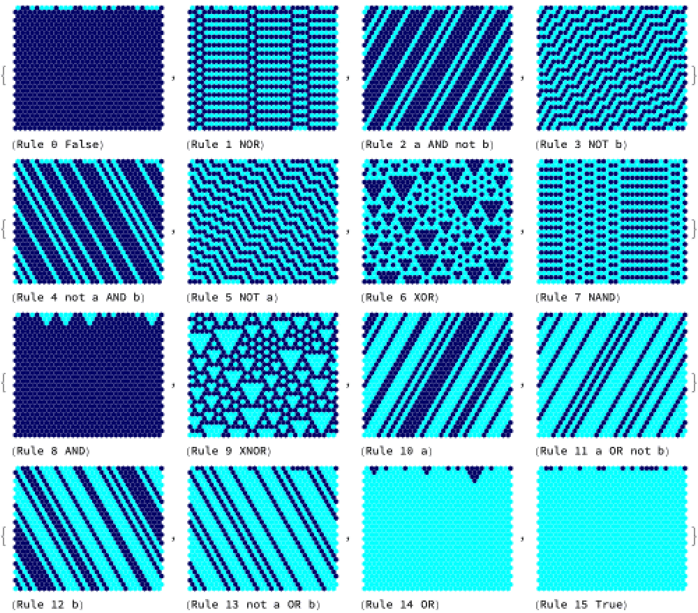
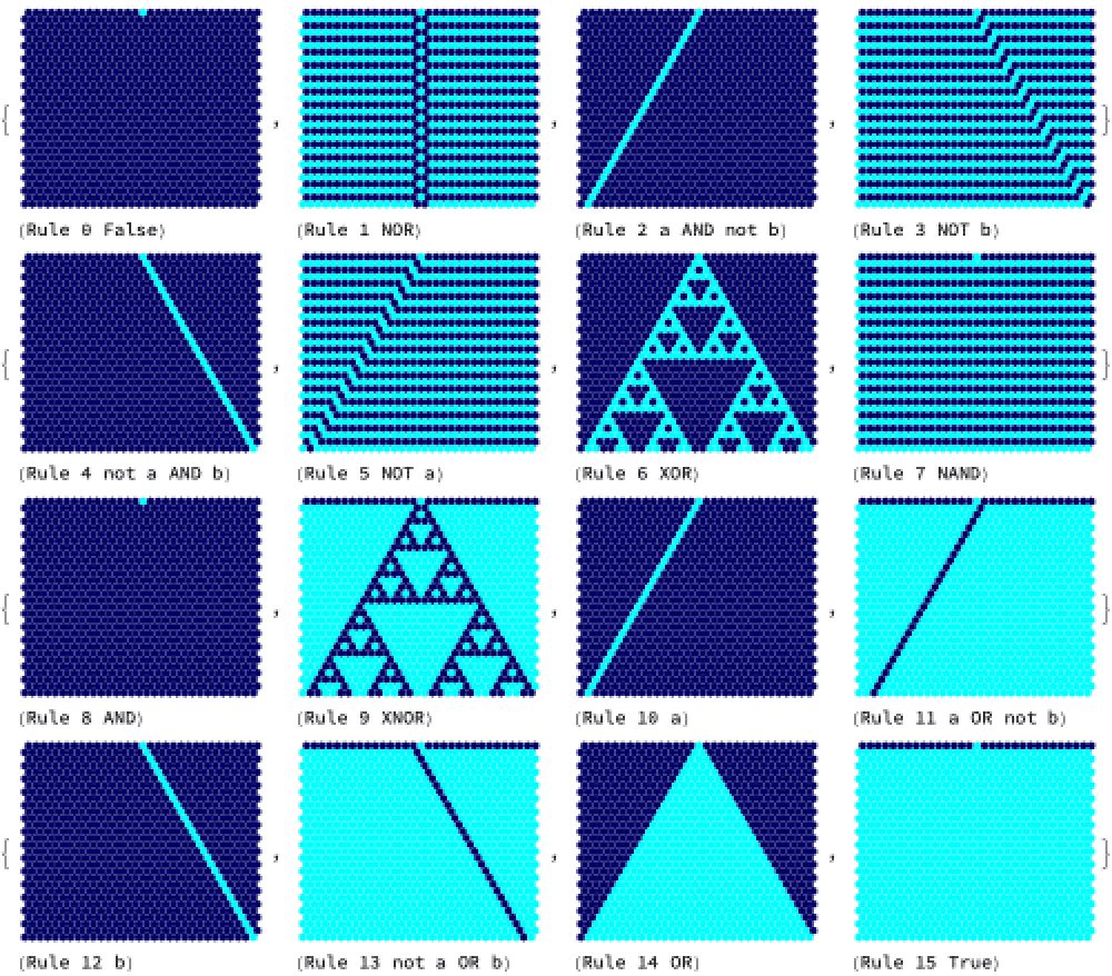
Since the hexagon tiling oriented with points up gives each cell only two neighbors, there are only 16 total rules. An interesting consequence of this is that it is very fast and easy to plot all of the rules and see what is happening all at once. Even more interestingly, each rule corresponds to one of the 16 binary logical connectives with two inputs.
Random Initial Conditions
Random Initial Conditions
Random initial conditions give a sense for which rules are “dual” to each other.
Seeing random conditions highlights how XOR creates the same behavior as XNOR, if both the inputs and the output are inverted. This also applies to AND and OR. In fact, any rule set involving an AND gate exhibits the same behavior as its “dual” with an OR gate, with the truth values of the inputs and outputs all reversed.
In addition, replacing a with b switches the direction of particles and of the propagation of repetition.
These plots were generated with width 31, height 30, seed type 5 (random), and tiling type 6. Rules 0 (top left) through 15 (bottom right) were generated.
Single Live Cell Initial Conditions
Single Live Cell Initial Conditions
Setting the initial conditions to a single living cell makes the behavior of most rules easier to understand.
Most of the rules output only a particle, repetition, or nesting (Sierpinski Triangle / Gasket)
Most of the rules output only a particle, repetition, or nesting (Sierpinski Triangle / Gasket)
Changing the seed type to 1 (single live cell).
Triangle Tiling (Some Edges Horizontal, 2 Cell Types, each with 5 neighbors)
Triangle Tiling (Some Edges Horizontal, 2 Cell Types, each with 5 neighbors)
Things started to get ugly when we started to analyze the triangle tiling. Not only are there infinitely many ways to divide it into rows (of which we only investigated two) but there are now also two distinct cell “types” due to the fact that different cells are rotated differently even in a single orientation of the tiling, and the differently rotated cells have different neighborhoods as defined by the row assignments and Moore neighborhoods. And the different orientations of the triangle tiling naturally have different cell “type” distribution, with the horizontal triangle tiling having alternating rows and the vertical triangle tiling having a “checkerboard” of cell types alternating both in rows and in columns. Since all 4 cell “types” in the two orientations had exactly 5 neighbors, we decided to keep rule setting to a single 5 digit number for both triangle grid orientations.
4 Billion
4 Billion
This plot was generated with width 31, height 30, seed type 1 (single cell), tiling type 4, and rule numbers Table[Floor[(n-1)*(2^(2^5)-1)/(16-1)], {n, 1, 16}] in order to go from Rule 0 to Rule 4294967295 in one sweep.
Triangle Tiling (Some Edges Vertical, 2 Cell Types, each with 5 neighbors)
Triangle Tiling (Some Edges Vertical, 2 Cell Types, each with 5 neighbors)
Things continued to be ugly with the triangle tiling rotated 60°.
More arbitrary rule sets
More arbitrary rule sets
The automata seem to behave similarly on both triangle tilings, however, unlike the case of the horizontal hexagon and diagonal square grids, the neighborhoods in the two triangle tilings are not identical. However the quantity of neighbors (5) and the arrangement of neighbors (more-or-less left-to-right) are similar in both tilings, partially explaining their similar behavior.
The same plot from above generated with width 31, height 30, seed type 1 (single cell),, and rule numbers Table[Floor[(n-1)*(2^(2^5)-1)/(16-1)], {n, 1, 16}] but with tiling type 3 instead of 4.
Concluding remarks
Concluding remarks
This project yielded interesting results, as we anticipated. In the future I may implement a way to animate the automata, generating one row at a time. I may also try to implement a way to input any tiling at any orientation and have the program divide it into rows and neighborhoods based on the cells’ y-coordinates, and then iterate an input rule on that tiling.
Keywords
Keywords
◼
Automaton
◼
Automata
◼
Tiling
◼
Tessellation
◼
Hexagon
◼
Triangle
◼
Fractal
Acknowledgment
Acknowledgment
I thank both my mentor Markus van Almsick and my co-mentor Bradley Klee for providing support and being overall enthusiastic about the project. I also thank Stephen Wolfram for the original idea.
References
References
◼
Wolfram, Stephen. A New Kind of Science. Wolfram Media, 2019.