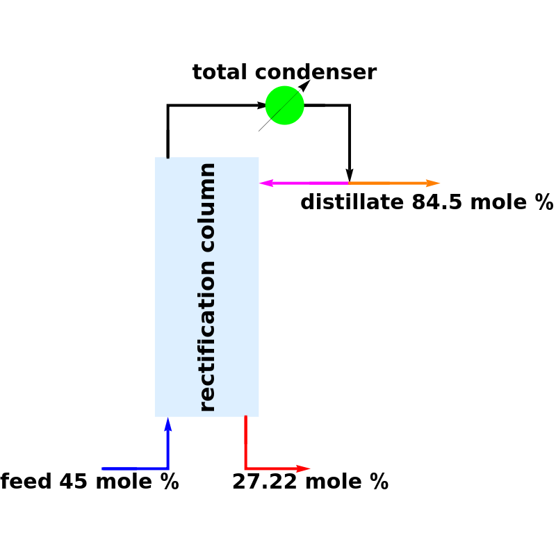
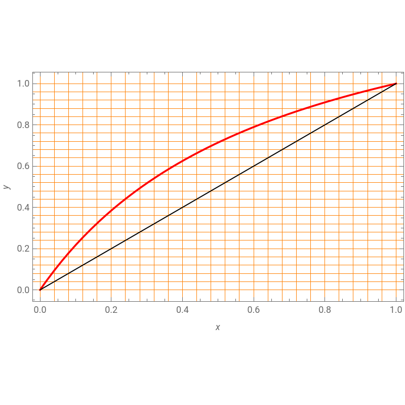
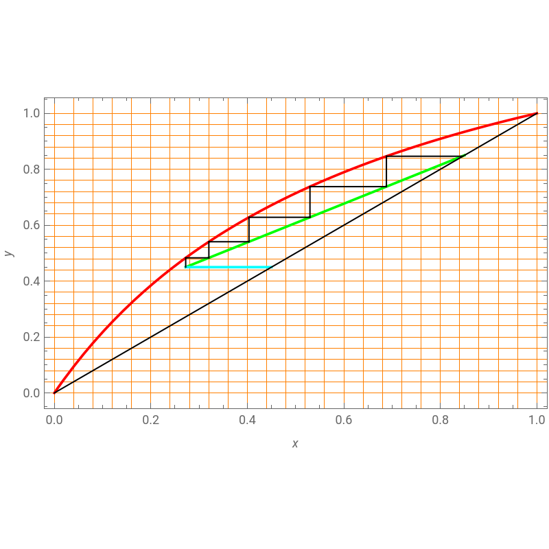
Consider a feed containing a binary mixture of compounds A and B with 45 mole % of the lighter component. This feed is a saturated vapor, which will be enriched in a rectifying column in order to obtain a distillate with 85 mole % purity. Enriching or rectifying columns are used when a pure bottom is not needed. This notebook displays the McCabe–Thiele graphical construction for a reflux ratio = 2.25, relative volatility = 2.5, and maximum number of stages = 5. The actual number of stages will be equal or less than the maximum number of stages value. You can easily see if the distillate specification has been reached or not. In addition, the composition of the liquid stream that exits at the bottom of the rectifying column is computed and given in the set-up figure.
In[]:=
α=2.5;(*constantrelativevolatilitymixture*)eq[x_]:=;(*plotofequilibriumcurve*)plt1=Plot[eq[x],{x,0,1},PlotStyle{RGBColor[1,0,0],Thickness[0.005]},Epilog{Black,Line[{{0,0},{1,1}}]},FrameTrue,FrameLabel{x,y},GridLinesStyleDirective[Orange],ImageSize{400,400},GridLines{Table[i,{i,0,1.0,0.04}],Table[i,{i,0,1.0,0.04}]}]
αx
x(α-1)+1
Out[]=
In[]:=
rect[x_]:=x+xD;(*operatinglineforrectifyingsection*)xD=0.85;(*distillatepurityspecification*)R=2.25;(*refluxratio*)
R
R+1
1
R+1
In[]:=
feed[x_]:=x-;(*feedlineequation*)q=0.0;(*feedissaturatedvapor*)zf=0.45;(*feedcomposition*)
q
q-1
zf
q-1
In[]:=
sol1=Solve[rect[x]feed[x],x];xu[1]=First[x/.sol1];yu[1]=rect[xu[1]];(*intersectionpointofoperatinglineandfeedline*)
In[]:=
plt2=Plot[rect[x],{x,xD,xu[1]},PlotStyle{RGBColor[0,1,0],Thickness[0.005]}];
In[]:=
plt3=Plot[feed[x],{x,zf,xu[1]},PlotStyle{RGBColor[0,1,1],Thickness[0.005]}];
In[]:=
i=1;Np=5;(*maximumnumberofstages*)(*steppingoffstages*)While[i≤Np&&xu[i]≤xD,{yu[i+1]=eq[xu[i]],sol=FindRoot[rect[t]yu[i+1],{t,0.5}],xu[i+1]=t/.sol,i++}];iu=i-1;
In[]:=
xu[iu+1]
Out[]=
0.845036
In[]:=
(*McCabe&Thieleconstruction*)Show[plt1,plt2,plt3,Graphics[{Table[Line[{{xu[i],yu[i]},{xu[i],yu[i+1]}}],{i,1,iu}],Table[Line[{{xu[i],yu[i+1]},{xu[i+1],yu[i+1]}}],{i,1,iu}]}],ImageSize{400,400}]
Out[]=
In[]:=
(*columnset-up*)Show[Graphics[{LightBlue,Rectangle[{0,0},{4,10}],Thick,Blue,Arrow[{{-2,-2},{0.5,-2},{0.5,0.}}],Red,Arrow[{{3.5,0.},{3.5,-2},{6,-2}}],Thick,Black,Arrow[{{0.5,10},{0.5,12},{4.5,12}}],Arrow[{{5.5,12},{7.5,12.0},{7.5,9.0}}],Magenta,Arrow[{{7.5,9.0},{4.0,9.0}}],Orange,Arrow[{{7.5,9.0},{11.0,9.0}}],Green,Disk[{5.0,12},0.75],Black,Thin,Arrow[{{4.,11},{6.0,13.0}}],Rotate[Style[Text["rectification column",{2,5},{0,0}],Black,Bold,16],Pi/2],Style[Text["total condenser",{5,13.25},{0,0}],Black,Bold,15],Style[Text["distillate 84.5 mole %",{10.5,8.25},{0,0}],Black,Bold,15],Style[Text["feed 45 mole %",{-2.5,-2.5},{0,0}],Black,Bold,15],Style[Text[ToString[SetPrecision[100xu[1],4]]<>" mole %",{6.0,-2.5},{0,0}],Black,Bold,15]}],ImageSize{400,400}]
Out[]=