In this project, the impact of scaling weights, shifting biases, and swapping activation functions on re-trained neural network accuracy is explored. The project asks if there a possibility that manipulating the parameters of a trained network post-training can let the network fit the training data in a slightly different way, to potentially even increase the accuracy of the network once it’s then retrained. LeNet is the model chosen for these explorations for its relatively simpler structure, which helped code run faster, and available training data. The results of the explorations suggest that it is actually possible to find a better accuracy for a neural net by going through this weight modification and retraining process with specific numbers (in this essay, numbers specific to LeNet). The effect is not as great when only specific layers’ weights are modified. Additionally, more exploration would be needed on biases and activation functions to see their potential for increasing accuracy when combined in certain ways, with the activation function being similar to the original ReLU if the shifts in biases should go into negative values.
Introduction
Introduction
Neural networks are useful machine learning models made of layers of interconnected neurons, each applying a linear transformation (via weights and biases) followed by a non-linear activation function. These parameters (the weights and biases) control how input features influence the output, and are continuously learned and updated during training to minimize the network’s loss.
The starting idea for this exploration comes from the loss graph for the training of a neural net. Usually diagrams will show a curve that resembles a parabola with a minimum that you are trying to find through training the network. However, what if beyond this curve, there was another point where the loss was even smaller? If we could somehow kick the training process beyond the hill between the 2 minimums, it would increase the accuracy of the model, but instead of editing our way of descending the hill, what if we edited our starting point in such a way that we would end up in a different minimum? This is why in this exploration the pre-trained weights are then modified in hopes that retraining will produce a different, better result.
The starting idea for this exploration comes from the loss graph for the training of a neural net. Usually diagrams will show a curve that resembles a parabola with a minimum that you are trying to find through training the network. However, what if beyond this curve, there was another point where the loss was even smaller? If we could somehow kick the training process beyond the hill between the 2 minimums, it would increase the accuracy of the model, but instead of editing our way of descending the hill, what if we edited our starting point in such a way that we would end up in a different minimum? This is why in this exploration the pre-trained weights are then modified in hopes that retraining will produce a different, better result.
Previous work
Previous work
Last year, there was a student who applied different kinds of parameter changes to the four layers in LeNet to find out how sensitive the network is to noise and which layers, when perturbed, have the most impact on the output of the net. Another was exploring what exactly would happen to the network and its comparative performance if he specified different kinds of weight initializations for the untrained network.
More generally, the type of exploration being done is in a way related to studies on the robustness of networks, in the sense that the weights of a neural network are being changed again post-training so the effects on later outputs can be observed. Additionally, a lot of work has been done in trying to minimize loss in better ways through tweaks to gradient descent during the training of a network, by introducing some element of randomness to help it over some local minima. What I’m wondering is if there is a possibility that something at least a little similar can be done with weight perturbations on a trained network, then training and updating its weights again.
More generally, the type of exploration being done is in a way related to studies on the robustness of networks, in the sense that the weights of a neural network are being changed again post-training so the effects on later outputs can be observed. Additionally, a lot of work has been done in trying to minimize loss in better ways through tweaks to gradient descent during the training of a network, by introducing some element of randomness to help it over some local minima. What I’m wondering is if there is a possibility that something at least a little similar can be done with weight perturbations on a trained network, then training and updating its weights again.
LeNet model
LeNet model
LeNet, a convolutional neural network for image classification, was released in 1998 by Yann LeCun and his besties at AT&T Bell Labs. It was developed during machine learning experimentation with the goal of being able to classify the MNIST dataset, or to identify the right handwritten digits in images, and it has been really successful, with the model’s accuracy reported as almost 98.5%. The trained network is taken directly from the Wolfram Neural Net Repository, along with the MNIST training data.
Getting LeNet from the repository:
In[]:=
lenetModel=NetModel["LeNet Trained on MNIST Data"]
Out[]=
NetChain


Layers/What’s inside
Layers/What’s inside
From the NetChain it can be seen that LeNet has two convolutional layers and two linear layers. The network begins by taking a 28 by 28 grayscale image (of a handwritten digit) as input and proceeding through convolutional and pooling layers to capture its important features. This gives a feature map with dimensions 50 x 4 x 4. The resulting data is then reshaped into a 1 by 800 vector before passing through the other layers to get to the final classification (digits 0-9). The diagram below shows a better visual of the LeNet architecture:
Getting a graphic of what’s inside LeNet:
In[]:=
Information[NetModel["LeNet Trained on MNIST Data"],"SummaryGraphic"]
Out[]=

MNIST
MNIST
The MNIST data mentioned is a database of handwritten digits that is commonly used for training image processing systems. It contains 60,000 28 by 28 grayscale images for its training data and 10,000 images of the same sort for its testing data.
Getting both the MNIST training data and test data from the repository:
trainingData=ResourceData["MNIST","TrainingData"];testData=ResourceData["MNIST","TestData"];
Take a sneak peek of what’s inside:
In[]:=
RandomSample[trainingData,5]
Out[]=
9,

8,

7,

0,

4

Making associations for training and test data (Separating the keys and values to get separate lists of input vs. target):
bigtrainAssoc=<|"Input"Keys[trainingData],"Target"Values[trainingData]+1|>;bigtestAssoc=<|"Input"Keys[testData],"Target"Values[testData]+1|>;
Take a sneak peek:
Take[bigtrainAssoc,All,5]
Out[]=
Input
,

,

,

,

,Target{1,1,1,1,1}

The Existing Weights
The Existing Weights
Just to see what kind of values there already are in the weights of the original LeNet:
Get numeric arrays of the weights of each of the 4 layers with weights in LeNet:
In[]:=
existingWeights=Quiet[Select[NetExtract[lenetModel,{All,"Weights"}],NumericArrayQ[#]&]]
Out[]=
NumericArray,NumericArray,NumericArray
,NumericArray

Get a sneak peek at some of the weights in the first layer of LeNet:
In[]:=
(existingWeights[[1]]//Normal)[[1]]
Out[]=
{{{-0.167045,-0.369549,-0.612365,-0.531681,-1.5101},{-0.636221,-0.41981,-0.261644,-0.105551,-0.701257},{-0.0159123,0.321061,-0.198172,-0.556536,-0.75463},{-0.0189375,-0.335424,-0.376416,-0.367631,-0.981514},{0.580164,-0.581963,-0.180054,0.0422878,-0.29461}}}
Get a sneak peek at some of the weights in the second layer of LeNet :
In[]:=
(existingWeights[[2]]//Normal)[[1]][[1]]
Out[]=
{{-0.0232202,-0.11293,0.0186209,-0.0213377,-0.007215},{0.0286192,-0.119415,0.0240125,-0.116497,0.0673954},{0.0436027,0.0208235,-0.0933471,0.0295251,-0.0543261},{0.0423229,-0.0143726,0.0782676,-0.0605527,-0.152211},{0.0216736,-0.00622586,0.0701731,-0.0957244,-0.143811}}
Get a sneak peek at some of the weights in the third layer of LeNet :
In[]:=
Take[((existingWeights[[3]]//Normal)[[1]]),25]
Out[]=
{-0.107479,-0.00315954,-0.00135298,0.0345921,0.131435,-0.0697601,-0.12132,0.00191235,0.126075,0.0196901,0.0778908,0.00419545,0.12726,0.0286008,0.0987875,-0.103214,-0.109095,0.0769393,-0.167283,-0.229013,0.000958951,0.127575,-0.320556,-0.0237612,-0.0421318}
Get a sneak peek at some of the weights in the fourth layer of LeNet :
In[]:=
Take[((existingWeights[[4]]//Normal)[[1]]),25]
Out[]=
{-0.180276,-0.0321327,-0.404099,-0.103857,-0.160154,0.16109,0.125073,0.0294418,-0.0716324,0.0251843,0.125505,0.027618,-0.483546,0.11301,0.000691322,-1.06706,0.29167,0.191121,-0.606527,-0.0335045,-0.133701,0.1025,0.105827,0.488706,0.0513204}
I plan to, as a first step, multiply every weight by 2 and then retrain, and the results from that will be talked about later in the essay.
Accuracy to Compare to
Accuracy to Compare to
For the later explorations in the essay, there needs to be something to compare newly found accuracies to, like some kind of starting point number. For this, I’ll first bring up the accuracy of LeNet from the repository.
Measure the accuracy of the repository’s LeNet on its test data:
In[]:=
oldAcc=ClassifierMeasurements[lenetModel,testData,"Accuracy"]
Out[]=
0.9848
Another thing that follows is that if the weights of the network are to be adjusted and then the network to be retrained, we should check the accuracies of both directly retraining the original network and multiplying the weights by 1 and retraining.
Original Network :
Construct the NetGraph to be used for retraining the original model:
trainingOrigModel=NetGraph[<|"lenet"lenetModel,"loss"CrossEntropyLossLayer["Index"]|>,{NetPort["Input"]"lenet"NetPort["loss","Input"],NetPort["Target"]NetPort["loss","Target"]}]
Out[]=
NetGraph

Making a smaller dataset to train on, of 10,000 training images and 2,000 testing images (reasoning is explained in the section below):
smalltrainingdata=RandomSample[trainingData,10000];smalltestdata=RandomSample[testData,2000];
Making associations for small training and test data and separating the keys and values to get separate lists of input vs. target:
trainAssoc=<|"Input"Keys[smalltrainingdata],"Target"Values[smalltrainingdata]+1|>;testAssoc=<|"Input"Keys[smalltestdata],"Target"Values[smalltestdata]+1|>;
Train the net and save the results:
resultOrigModel=NetTrain[trainingOrigModel,trainAssoc,All,ValidationSettestAssoc,MaxTrainingRounds5,TargetDevice"CPU"]
Out[]=
NetTrainResultsObject

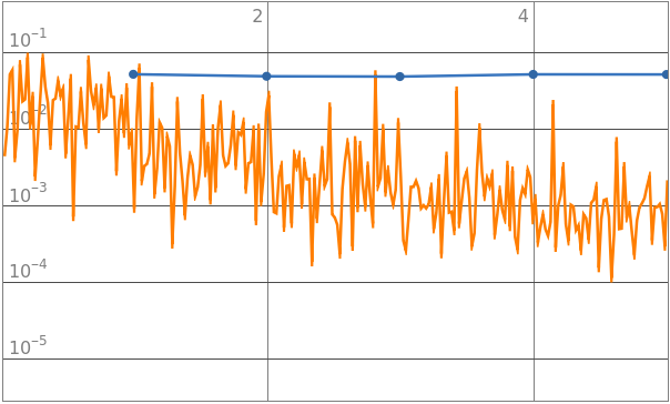
Extract the new net from the results:
Define the encoder (image to numbers) and decoder (digit from numbers):
Put back the encoder and decoder:
Measure the accuracy of the network now:
Original Network, with weights x 1:
Scaling all the weights of the original model by 1:
Constructing the NetGraph used to train the net:
Train the net and save the results:
Extract the trained net from the results object:
Put back the encoder and decoder:
Get the accuracy of the retrained model:
It seems that the accuracies are the same, which is good.
Explorations
Explorations
While all the explorations below are done with the LeNet model, a lot of the code was written with the Inception V3 model in mind instead. I had changed to LeNet because the MNIST training and testing data was already available within the repository. The network was also a lot less complicated, which helped with the amount of time needed to run each exploration.
The explorations below were also generally not pre planned, but rather thought of one after the other in some order, based on the results from previous explorations. As a starting point, I first went in and multiplied every weight in the network by 2, just to see what would happen to its accuracy.
Common Functions Used
Common Functions Used
A function that, given a layer, returns a new layer with all the original weights multiplied by 2 (parameter has to be a layer with weights):
Function that, given a net, returns a new net in which all layers with weights in the original net have been replaced with their scaled counterparts:
Scaling All Weights By 2
Scaling All Weights By 2
For this one, since it was a starting point for the rest of these explorations, I used the full 60,000 images in the training data. I took the original LeNet and directly scaled its weights by 2, then retrained it.
(First, I list out all the lines of code used in the new net functions and explain them. Then, I use the defined function to continue with the net training.)
Define a list of the layers in LeNet:
Make an association between the layer indexes and the actual layers themselves:
Get the association of layers, except with their weights all scaled by 2:
Collect the keys of that association:
Define a new network, in which all layers with weights are replaced with their scaled counterparts from the association:
Check the accuracy of the untrained model, just out of curiosity:
Compare the old (LeNet) and new (LeNet x 2, untrained) accuracies:
Here it is seen that the scaled net is immediately at a lower accuracy than the original. What happens when it is retrained?
Use the getNewNet function to quickly scale the weights of a net by 2:
Define the NetGraph used to begin training the network, using a Cross Entropy Loss Layer:
Train and get the results of training the scaled network:
Extract the now trained scaled net from the training results:
Attach the encoder and decoder back onto the network:
Get the new accuracy, after training, of the scaled net:
Surprisingly, the accuracy turns out greater than the original 0.9848 of LeNet, an improvement made just by scaling the weights.
Because of this weird increase in accuracy, I decided to run the same process on the network, but over a range of numbers (to scale with) to see if there is something visually interesting about the accuracies once plotted. At what point would it start to decrease the accuracy of the network, once retrained?
Using a Smaller Dataset
Using a Smaller Dataset
However, the problem with experimenting over a range of scaling factors and training them is the amount of time needed to run the code. In the previous section, training on the 60,000 images took about 30 minutes, which by itself is not that bad, but is also not great if you need to run that 5 times.
I decided to use a smaller dataset (briefly mentioned, in a previous section), reducing the 60,000 training images to 10,000, and the 10,000 testing images to 2,000. This results in a training time of between roughly 3 to 10 minutes each, which was very useful for this section!
{0.5, 1.0, 1.5, 2.0, 2.5}
{0.5, 1.0, 1.5, 2.0, 2.5}
I picked these 5 numbers to begin with, all close to 2 and incrementing by 0.5 every time. I also updated my layer weight scaling function to include another useful parameter:
Function that, given a layer with weights, returns that layer except with its weights scaled by num:
Then I updated the function for getting a new scaled network to include that parameter as well.
Function that, given a net, returns a new net in which all layers with weights in the original net have been replaced with their new scaled (by factor of num) layers:
Define an association of a range of scaling factors, each to be used on a different net:
Define an association of a range of scaling factors, each to be used on a different net:
For the whole association, replace the values with newly scaled nets:
For the whole association, construct the NetGraphs with which the networks will train:
For the whole association, train the networks to get the results objects:
Extract all the networks from the training results:
Attach the encoders and decoders again, for every net:
Get the accuracies of the nets:
The only reason the net10 (network x 1) accuracy is a bit different than in the previous section is because after quitting the kernel, the training set was RandomSampled again. But since the range of numbers were computed the same way as each other, the comparisons are still okay.
Get a plot of the accuracies:
After seeing this plot, I was wondering why the accuracy of scaling by 2 was a lot less than the others, especially the accuracy after retraining virtually the same model. This is why I realized I needed to compare to the accuracy after retraining the original model too.
I decided to zoom in around the accuracy point for scaling the network by x1 (and after x 2.5) to see where the graph goes (up or down) on both sides.
Adding Points In between
Adding Points In between
Define an association of a range of scaling factors, each to be used on a different net:
For the whole association, replace the values with newly scaled nets:
For the whole association, construct the NetGraphs with which the networks will train:
For the whole association, train the networks to get the results objects:
Extract all the networks from the training results:
Attach the encoders and decoders again, for every net:
Get the accuracies of the nets:
Get the graph of all the previously calculated accuracies:
It turns out that there actually is a value for which the scaled and retrained network does better in accuracy than the original one! When all the weights are scaled by 0.75, the accuracy increases to 0.989.
I was very surprised, so I decided to add even more points on the other side of 4.0 in the graph, up to 6.0 and even 10.
Define an association of a range of scaling factors, each to be used on a different net:
For the whole association, replace the values with newly scaled nets:
For the whole association, construct the NetGraphs with which the networks will train:
For the whole association, train the networks to get the results objects:
Extract all the networks from the training results:
Attach the encoders and decoders again, for every net:
Get the accuracies of the nets:
Get a plot of all previously calculated accuracies:
Since that didn’t give points that were as interesting as 0.75, I decided to zoom into a different part of the graph, the parts closer to 0.75 (0.6, 0.65, 0.7, 0.8, 0.9), to see if you can go even higher than that. The process was the same.
Define an association of a range of scaling factors, each to be used on a different net:
For the whole association, replace the values with newly scaled nets:
For the whole association, construct the NetGraphs with which the networks will train:
For the whole association, train the networks to get the results objects:
Extract all the networks from the training results:
Attach the encoders and decoders again, for every net:
Get the accuracies of the nets:
Graph of the new accuracy points:
Graph of all previously calculated accuracy points:
From these, the accuracy calculated from scaling by 0.8 is highest, and is still higher than scaling by 1.0.
Other Layer Combos
Other Layer Combos
After experimenting with different scalings of weights for every weight in the network, I wanted to know what would happen to the accuracy if I only changed the weights of specific layers. Some places online said that the last layer of a network was one of the most important to its output, and previous student work had also gathered that convolution layers were more sensitive to perturbations than classification layers, so I wanted to see if that would do anything interesting.
Here I’ve scaled the weights of the fourth layer only by 0.8.
Define a new network by swapping out the 4th layer with weights with scaled a version of itself (by 0.8):
Construct the NetGraph to be used for retraining the updated net:
Train the net and save the results object:
Extract the new net from the training results:
Put back the network’s encoder and decoder:
Measure the accuracy of the new network:
It seems that the accuracy is not bad, but not as good as having the network be retrained with every weight having been scaled. This observation will actually continue for the next exploration as well.
Now I’ve scaled the weights of the first layer by 2 and the 4th by 0.8, just to see what would happen if I changed a convolutional and the last layer at the same time.
Define a new network by swapping out the 1st and 4th layers with weights with scaled versions of themselves (by 2 and 0.8):
Construct the NetGraph to be used for retraining the updated net:
Train the net and save the results object:
Extract the new net from the training results:
Put back the network’s encoder and decoder:
Measure the accuracy of the new network:
This time, it’s also not as good as the original network retrained. I will conclude that multiplying every weight in the network by a number is more effective than only selecting certain layers of the network to do this with.
What Happens With Biases
What Happens With Biases
After seeing what has happened when we change the weights of a network and retrain it, I wanted to see if similar things could be done with biases.
I altered the code from the weights explorations and repeated the process with biases:
Function that, given a layer with biases, returns a new layer in which the original biases are increased by num:
Function that, given a net, returns a new network in which all layers with biases have been replaced by new layers in which the original biases are increased by num:
Define an association of a range of biases to be added, each to be used on a different net:
For the whole association, replace the values with the nets with new biases:
For the whole association, construct the NetGraphs with which the networks will train :
For the whole association, train the networks to get the results objects:
Something interesting is happening inside the loss graphs for the negative bias shifts. I suspect that this is because of the network’s current activation function, or ReLU/Ramp, and its tendency to suppress negative input values.
Extract all the networks from the training results :
Attach the encoders and decoders again, for every net :
Get the accuracies of the nets :
Graph of the accuracies of the nets with changed biases:
(The difference between positive and negative bias shifts can also be seen here.)
I wondered what would happen if I did the same thing but with numbers that were closer to 0 and 2, whose nets’ accuracies seemed to be pretty high, if not the highest.
Defining a new range of biases to be added:
For the whole association, replace the values with new nets (with new biases):
For the whole association, construct the NetGraphs with which the networks will train:
For the whole association, train the networks to get the results objects:
Extract all the networks from the training results:
Attach the encoders and decoders again, for every net :
Get the accuracies of the nets:
Graph of the accuracies of the new retrained networks:
From here we can guess that just adding 0 to every bias in the network gets the highest accuracy (the original network). This is the reason why I won’t go and experiment with combinations of weights and biases, especially while using Ramp layers in LeNet.
Activation functions
Activation functions
I didn’t realize the issue with negative biases and the activation function before I did this section, but otherwise I would have just done combinations of different activation functions with the biases from before. The following are just 2 experiments with what would happen if all we changed in between training was the activation function (to Tanh[] & Swish[]).
Tanh:
Replace every activation layer with Tanh:
Construct the NetGraph to be used for retraining the updated net:
Train the net and save the results object:
Extract the new net from the training results :
Put back the network’s encoder and decoder:
Measure the accuracy of the new network:
The accuracy was really terrible compared to previously calculated values of the network’s accuracy. This was probably because the change in activation function literally changed how the network calculates the loss to update its weights during training. I suspect then that the change in activation function removes some of the advantage of already having the model’s pre-trained weights before altering them and retraining them. In any case, here’s Swish:
Replace every activation layer with Swish :
Scale the updated network by 0.8:
Construct the NetGraph to be used for retraining the newly updated net:
Train the net and save the results object:
Extract the new net from the training results :
Put back the network’s encoder and decoder:
Measure the accuracy of the new network:
The accuracy seems to now be closer to the previous explorations. One reason could be that the Swish function’s shape is significantly more similar to ReLU than Tanh’s, just dipping a little bit into negative values, which would not completely throw off the first training. Another is just the weight scaling factor, which also increases the accuracy of the network once retrained.
Now that I’m reflecting more about the process, I realize that exploring into combinations of negative and positive biases and different activation functions would probably be more effective with activation functions that look at least a little like the original one, ReLU.
Now that I’m reflecting more about the process, I realize that exploring into combinations of negative and positive biases and different activation functions would probably be more effective with activation functions that look at least a little like the original one, ReLU.
Conclusion
Conclusion
So far we’ve looked at different explorations of what would happen once we take a pre-trained model, mess around with its weights, and then retrain it, and whether it can even produce a better accuracy than before. From the results, it seems that there is such a possibility, as scaling the weights of a network by some number (in LeNet’s case, a number like 0.8) and training it again is actually able to raise its already pretty high accuracy. Additionally, scaling the weights on all layers instead of only specific layers (like 1st or 4th) is more effective for doing this sort of thing. I also found that shifting the biases and retraining the model doesn’t do anything as interesting as the weights example, and that especially with the ReLU activation function, the negative shifts don’t really work that well. Lastly, with activation functions, the closer the function was to the original one, the better the accuracy would be, especially combined with scaling the weights of the network. These results can be a starting point for future explorations for potentially increasing the accuracy of more networks and network retraining.
Future Work
Future Work
A big limitation on this exploratory project was the time limit of the program: some code needed time to run, and other pieces of code could not run simultaneously, so a lot of time was spent waiting or writing comments. If better hardware accelerators were available, more experiments could have been done, a few of which include exploring a similar approach to a network’s ability to do transfer learning, doing the same experiments on different neural nets (bigger ones too, like Inception V3), or doing more combinations of changing weights, biases, and activation functions all together (testing out the suspicions about both the negative biases and the impact of the similarity of the new activation function along the way).
CITE THIS NOTEBOOK
CITE THIS NOTEBOOK
Impact of post-training parameter modifications on a trained neural network
by Raeanne Li
Wolfram Community, STAFF PICKS, July 10, 2025
https://community.wolfram.com/groups/-/m/t/3501705
by Raeanne Li
Wolfram Community, STAFF PICKS, July 10, 2025
https://community.wolfram.com/groups/-/m/t/3501705