Quantum tensor networks are compact factored representations of many-body quantum states and operators using small tensors connected by contracted indices. Nodes are finite-rank tensors; edges are index pairings; open edges are physical degrees of freedom; internal edges are virtual bonds whose dimension controls expressiveness versus cost. For more details, please refer to Wolfram quantum framework’s documentation page for tensor networks.
We adopt the following conventions. We write tensors using the notation . In diagrammatic tensor networks, upper (contravariant) indices are treated as outputs and lower (covariant) indices as inputs. Upper indices correspond to vector components (kets), while lower indices correspond to covector components or linear functionals (bras). The domain of a tensor is represented by its input legs (lower indices), and the codomain by its output legs (upper indices).
output
input
Given a vertex of a directed graph, any edge represents a contraction. The incoming edges correspond to input indices and outgoing ones to output indices.
For contraction, we shall use Einstein summation which requires tensors, their indices, and optionally the set of output indices. The convention is that repeated indices are summed over, and if necessary the resulting tensor is transposed according to the specified outputs. The syntax is EinsteinSummation[indices->out,tensors]. This implementation is a modified version of the WFR function. EinsteinSummation transforms the summations into Mathematica expressions (e.g., TensorContract) that are much more efficient than manually summing over indices.
Install quantum framework paclet (we shall use only some of tensor network features)
In[]:=
PacletInstall["https://www.wolfr.am/DevWQCF",ForceVersionInstall->True]<<Wolfram`QuantumFramework`
Out[]=
PacletObject

Recipe to convert a directed acyclic graph into a tensor network
Recipe to convert a directed acyclic graph into a tensor network
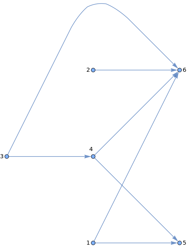
Generate a random acyclic directed graph:
In[]:=
g=DirectedGraph[RandomGraph[{6,7}],"Acyclic",VertexLabels->v_:>HoldForm[v],GraphLayout->{"LayeredDigraphEmbedding","Orientation"->Left}]
Out[]=
Get the list of vertexes and edges:
In[]:=
v=VertexList[g];e=EdgeList[g];
Generate an empty association with keys as vertexes and values empty list (vertex->{})
In[]:=
empty=AssociationThreadVertexList[g]->s./.s.->{};
Generate the vertex-edge incidence matrix of the graph (+1 entries are incoming edges and -1 are outgoing ones)
In[]:=
inm=IncidenceMatrix[g];ps=inm["ExplicitPositions"];vl=inm["ExplicitValues"];
Generate an association in the form with indices are enumerated using their order in the edge list:
vertex->{{listofinputindices},{listofoutputindices}}
In[]:=
inputOut=Merge[{Join[empty,<|#[[1,1]]->#[[All,2]]&/@GatherBy[Pick[ps,vl,1],First]|>],Join[empty,<|#[[1,1]]->#[[All,2]]&/@GatherBy[Pick[ps,vl,-1],First]|>]},Identity]
Out[]=
1{{},{1,2}},2{{},{3}},3{{},{4,5}},4{{4},{6,7}},5{{1,6},{}},6{{2,3,5,7},{}}
Put together all indices per vertex:
In[]:=
indices=Catenate/@Values@inputOut
Out[]=
{{1,2},{3},{4,5},{4,6,7},{1,6},{2,3,5,7}}
The length of each sublist can be understood as rank of each tensor at a given vertex:
In[]:=
Length/@indices
Out[]=
{2,1,2,3,2,4}
Given a maximum dimension, randomly assign a dimension between 2 to max dimension to every index:
In[]:=
maxDim=4;indexDim=AssociationThread[DeleteDuplicates@Catenate@indices->RandomInteger[{2,maxDim},Length@DeleteDuplicates@Catenate@indices]]
Out[]=
14,24,33,42,54,63,73
Now for each tensor/vertex, we have a list of indices and their dimensions. So one can generate corresponding tensors. We shall do it by randomly generating complex-valued tensors:
In[]:=
tensorsN=RandomComplex[{-1-I,1+I},#]&/@(indices/.Normal[indexDim]);
Now given indices, do the contraction (note that repeated indices mean the summation is done over them)
In[]:=
out1=EinsteinSummation[indices,tensorsN]//ActivateTensor
Out[]=
21.07-1.39323
Tensors can be defined as symbolic objects and not being defined explicitly. The only info that we shall include will be their dimensions. We shall discuss this unique feature in another post when we will discuss different methods to find optimal contraction path.
Given definitions, define tensors symbolically:
In[]:=
tensorsSym=ArraySymbol[Unique["T"],#]&/@(indices/.Normal[indexDim]);
Execute the tensor contraction:
In[]:=
EinsteinSummation[indices,tensorsSym]//ActivateTensor
Out[]=
TensorContract,{{1,9},{2,11},{3,12},{4,6},{5,13},{7,10},{8,14}}
T31
T32
T33
T34
T35
T36
It might be useful to include the information of input vs output into the index notation. To do that, in the Wolfram quantum framework, we have adopted covariant and contravariant convention. The upper (contravariant) indices are treated as outputs and lower (covariant) indices as inputs.
upper/contravariant index: output
lower/covariant index: input
upper/contravariant index: output
lower/covariant index: input
In[]:=
newIndices=AssociationThread[EdgeList[g]->Values@GroupBy[Transpose[{Flatten[KeyValueMap[{Table[Subscript[#1,j],{j,#2[[1]]}],Table[Superscript[#1,j],{j,#2[[-1]]}]}&]@inputOut],Flatten@Values[inputOut]}],Last->First]]
Out[]=
15{,},16{,},26{,},34{,},36{,},45{,},46{,}
1
1
5
1
2
1
6
2
3
2
6
3
4
3
4
4
5
3
6
5
6
4
5
6
7
4
6
7
We can put together all these info into our graph as annotation; basically creating an annotated graph, with tensor and index information where indices are properly formatted as upper/lower ones.
In[]:=
tn=Graph[MapThread[Annotation[#1,"Tensor"->#2,"Index"->#3]&,{Range[Length@tensorsN],tensorsN,Catenate/@KeyValueMap[{Table[Subscript[#1,j],{j,#2[[1]]}],Table[Superscript[#1,j],{j,#2[[-1]]}]}&][inputOut]}],EdgeList[g]/.DirectedEdge[x_,y_]:>DirectedEdge[x,y,newIndices[DirectedEdge[x,y]]],VertexLabels->Automatic,GraphLayout->{"LayeredDigraphEmbedding","Orientation"->Left}];
This convention is how we check for a tensor network in the Wolfram quantum framework:
In[]:=
TensorNetworkQ[tn]
Out[]=
True
Given a tensor network, ContractTensorNetwork (yet to be documented) automatically determines how contractions are performed from the network input. The procedure follows the same rules as the Einstein summation convention described previously.
Execute the contractions over the tensor network:
In[]:=
out2=ContractTensorNetwork[tn]
Out[]=
21.07-1.39323
Check the result is the same as before
In[]:=
out1-out2//Chop
Out[]=
0
Adding more legs/indices into tensors randomly
Adding more legs/indices into tensors randomly
In the previous section, the number of indices for each tensor was restricted to the number of edges connected to it. For a tensor network, tensors may contain additional indices, while edges correspond only to those to be contracted. The following defines a function that randomly adds indices to each tensor.
Given an initial index list of the form {in, out}, randomly add elements to either in or out. The maximum number of elements to be added is chosen randomly up to the value specified by the final argument. If the final argument is not given, the default maximum is one.
In[]:=
randomLegAddition[{in_,out_},add_:1]:=Module[{moreInput,moreOutput},{moreInput,moreOutput}=RandomInteger[add,2];{Join[in,Table[Unique["Leg"],moreInput]],Join[out,Table[Unique["Leg"],moreOutput]]}]
Add indices randomly to the previous index list:
In[]:=
inputOut2=randomLegAddition/@inputOut
Out[]=
1{{},{1,2}},2{{Leg37},{3,Leg38}},3{{},{4,5,Leg39}},4{{4,Leg40},{6,7}},5{{1,6},{Leg41}},6{{2,3,5,7,Leg42},{}}
Put together the new list of indices:
In[]:=
indices2=Catenate/@Values@inputOut2
Out[]=
{{1,2},{Leg37,3,Leg38},{4,5,Leg39},{4,Leg40,6,7},{1,6,Leg41},{2,3,5,7,Leg42}}
New rank of tensors:
In[]:=
Length/@indices2
Out[]=
{2,3,3,4,3,5}
Identify the free indices (which are the ones we added randomly):
In[]:=
freeIndices=Complement[Catenate[#],Catenate@indices]&/@Transpose[Values@inputOut2]//Reverse//Catenate
Out[]=
{Leg38,Leg39,Leg41,Leg37,Leg40,Leg42}
Given a maximum dimension, assign random dimensions to the newly added indices.
In[]:=
maxDim=3;indexDim2=AssociationThread[DeleteDuplicates@Catenate@indices2->RandomInteger[{2,maxDim},Length@DeleteDuplicates@Catenate@indices2]]
Out[]=
13,22,Leg372,33,Leg383,42,52,Leg393,Leg403,62,72,Leg412,Leg423
Generate tensor as complex-valued array given their dimensions randomly:
In[]:=
tensorsN2=RandomComplex[{-1-I,1+I},#]&/@(indices2/.Normal[indexDim2]);//AbsoluteTiming
Out[]=
{0.000037,Null}
Execute the tensor contraction and re-arrange the results based on the free indices:
Generate the corresponding tensor network:
Generate the corresponding index graph of tensor network and highlight each tensor by a different color (TensorNetworkIndexGraph is another function of Wolfram quantum framework for tensor networks, still not documented though!):
Test the new tensor network:
Double check that the free indices we added randomly is the same as those obtained automatically from the new tensor network (TensorNetworkFreeIndices is another function of the Wolfram quantum framework for the tensor networks, though still not documented!):
Contract the tensor network:
Check the results are the same:
Tensor networks from a quantum circuit
Tensor networks from a quantum circuit
In this section, we shall briefly review tensor networks in the Wolfram quantum framework and how quantum circuits can be converted into tensor networks.
Generate a quantum circuit:
Show its diagram:
Generate its corresponding tensor network:
Get the contraction path from the tensor network:
Get all indices:
One can get the indices list from TensorNetworkIndices function too (still not documented):
Replace indices that should be contracted, so the repeated indices are explicit:
Find free indices in the right order:
One can get free indices using TensorNetworkFreeIndices too (still not documented):
Get all tensors:
One can get all tensors using TensorNetworkTensors too (still not documented):
Execute the contraction:
Of course, one can get the result directly using ContractTensorNetwork. Check the results are the same
Final comments
Final comments
At Wolfram’s Quantum team, we’re actively working on finding more efficient contraction paths. We’re also building integrations with platforms such as cuQuantum to deliver optimized contractions tailored to specific hardware and GPUs. While these features aren’t released yet, we already have strong support in place behind the scenes (for example, CUDA). We’d love to hear from you! If you’re interested in collaborating or have suggestions for how we can make these tools even more useful, please reach out to us at quantum AT wolfram.com
CITE THIS NOTEBOOK
CITE THIS NOTEBOOK
Symbolic tensor networks: from graphs to tensor networks
by Mohammad Bahrami
Wolfram Community, STAFF PICKS, September 22, 2025
https://community.wolfram.com/groups/-/m/t/3549258
by Mohammad Bahrami
Wolfram Community, STAFF PICKS, September 22, 2025
https://community.wolfram.com/groups/-/m/t/3549258