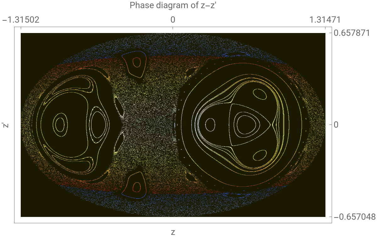
This is a slight improvement of the visualization of the dynamic system described in the following MSE link on Poincare Section of a Hamiltonian. I use ParallelTable and ArrayPlot to speed up the execution and visualization at the end. Also I add customized color function to indicate the distance between the point of interest and origin on the phase diagram in terms of .
{Z(t),Z'(t)}
Dynamic equation used in the MSE:
In[]:=
H[px_,pz_,x_,z_]:=1/2(px^2+pz^2)+z+2(3/4-Sqrt[x^2+(z-1)^2])^2-1/8xpp=D[x[t],t,t]-x[t](-4+3/Sqrt[x[t]^2+(-1+z[t])^2]);zpp=D[z[t],t,t]-3+3/Sqrt[x[t]^2+(-1+z[t])^2]-(-4+3/Sqrt[x[t]^2+(-1+z[t])^2])z[t];n=200;
In[]:=
TraditionalForm@Expand@{xpp==0,zpp==0}
Out[]//TraditionalForm=
(t)-++4x(t)0,-++++(t)+4z(t)-30
′′
x
3x(t)
2
x(t)
2
(z(t)-1)
3z(t)
2
x(t)
2
(z(t)-1)
3
2
x(t)
2
(z(t)-1)
′′
z
Parallel implementation
Parallel implementation
In[]:=
LaunchKernels[];
Slight modified the code on the MSE to take advantage of parallel programming:
In[]:=
res=ParallelTable[ics={Random[Real,{-0.55,0.55}],Random[Real,{-0.45,0.45}],Random[Real,{-0.44,0.9}],Random[Real,{-0.17,0.9}]};inisol=NSolve[H[ini,ics[[4]],ics[[1]],ics[[2]]]==0.866,ini];inival=ini/.inisol;ics={ics[[1]],ics[[2]],inival[[2]],ics[[4]]};TimeMin=0;TimeMax=14000;With[{Section=Reap[NDSolve[{xpp==0,zpp==0,x[0]==ics[[1]],z[0]==ics[[2]],x'[0]==ics[[3]],z'[0]==ics[[4]]},{x,z},{t,TimeMin,TimeMax},MaxSteps->∞,Method->{"EventLocator","Event"->x[t],"EventAction":>Sow[{z[t],z'[t]}]}]][[2]]},Transpose[Table[Section,{j,Length[Section]}]]],{i,1,n}];
During evaluation of In[8]:=
Extract the points for phase diagram plot:
In[]:=
pts=Flatten[res[[All,1,1]],1];
Find the farthermost point from the origin. I use this value to normalize the color map for all dots:
In[]:=
farAway=Max[Norm/@pts]
Out[]=
1.31505
Find the boundary for proper PlotRange
In[]:=
{minY,maxY}=MinMax[pts[[All,2]]];{minX,maxX}=MinMax[pts[[All,1]]];
In[]:=
coordToPixel//Clear
In[]:=
coordToPixel[pt_]:=Floor[{Rescale[pt[[2]],{minY,maxY},{1,960}],Rescale[pt[[1]],{minX,maxX},{1,960}]}]
Store pixel coordinates into a sparse array with customized default value for unspecified entries:
In[]:=
sa=SparseArray[Table[coordToPixel[ele]->Rescale[EuclideanDistance[ele,{0,0}],{0,farAway+0.1}],{ele,pts}],{960,960},1.];
The size of the data is about 2MB
In[]:=
Quantity,"Megabytes"
sa//ByteCount
1024.^2
Out[]=
Apply ColorData to encode the distance between dot in the phase diagram to origin: :
{z,z'}={0,0}
In[]:=
ArrayPlotsa,ColorFunction->(If[#>0.995,RGBColor@"#1a1a00",ColorData["TemperatureMap"][Mod[#+.3,1]]]&),AspectRatio,FrameLabel{{"z","Phase diagram of z-z'"},{"z'",None}},LabelStyle14,FrameTicks{{None,{{1,maxX},{480,0},{960,minX}}},{None,{{1,minY},{480,0},{960,maxY}}}}
1
GoldenRatio
Out[]=
Close the parallel subkernels to release memory:
In[]:=
CloseKernels[];
CITE THIS NOTEBOOK
CITE THIS NOTEBOOK
Visualization speed up for Poincare section of a Hamiltonian
by Shenghui Yang
Wolfram Community, STAFF PICKS, July 17, 2023
https://community.wolfram.com/groups/-/m/t/2967352
by Shenghui Yang
Wolfram Community, STAFF PICKS, July 17, 2023
https://community.wolfram.com/groups/-/m/t/2967352