We compute the three steady states of a diabatic continuous stirred tank reactor accomplishing an exothermic first order reaction. The study of the dynamics behavior for different initial conditions shows that two steady states, corresponding to the low and high conversions, are stable. On the other hand, the steady state corresponding to the intermediate value of the conversion is unstable.
Phase plane plot is given. Phase plane analysis confirms the conclusions concerning the steady states and shows that the unstable steady state is a saddle point. Temperature overshoot is observed. Knowing about possible overshoot behavior is a valuable information since temperature overshoot can lead to safety problems.
Acknowledgement: Numerical values were obtained from Ref. 1.
Dimensionless Governing Equations and dimensionless groups (see Refs. 1 and 2 for the derivation of these equations). Such equations are obtained from material and energy balance equations.
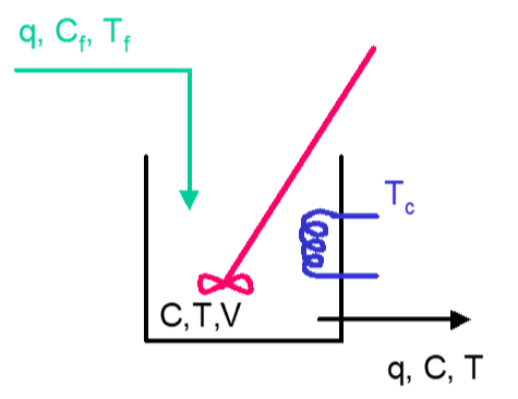
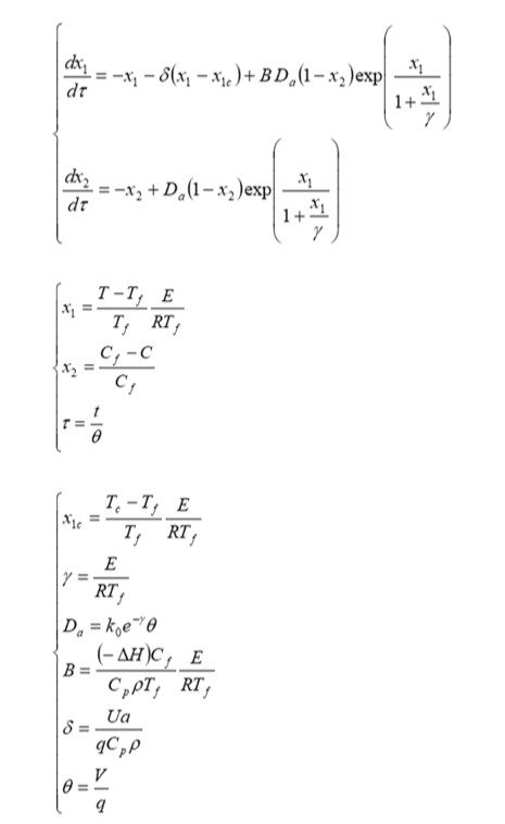
Numerical values are reproduced from Ref. 1
In[]:=
δ=150/500.;
In[]:=
γ=11834/(298.15 1.987);
In[]:=
D
a
In[]:=
B=5960 10/500 1/298.15 γ;
In[]:=
x
1c
Multiple steady states are found for the numerical values of γ, B, δ, and .
pt1 is the low temperature and low conversion stable steady state.
pt2 is the high temperature and high conversion stable steady state.
pt3 is the intermediate temperature and intermediate conversion saddle steady state.
x
1c
D
a
pt1 is the low temperature and low conversion stable steady state.
pt2 is the high temperature and high conversion stable steady state.
pt3 is the intermediate temperature and intermediate conversion saddle steady state.
In[]:=
root1=FindRoot[{-a1-δ(a1-)+B(1-a2)Exp[a1/(1+a1/γ)]0,-a2+(1-a2)Exp[a1/(1+a1/γ)]0},{a1,0.5},{a2,0.5}]
x
1c
D
a
D
a
Out[]=
{a10.946555,a20.154081}
In[]:=
pt1={a2,a1}/.root1
Out[]=
{0.154081,0.946555}
In[]:=
root2=FindRoot[{-a1-δ(a1-)+B(1-a2)Exp[a1/(1+a1/γ)]0,-a2+(1-a2)Exp[a1/(1+a1/γ)]0},{a1,5},{a2,0.8}]
x
1c
D
a
D
a
Out[]=
{a14.76533,a20.775705}
In[]:=
pt2={a2,a1}/.root2
Out[]=
{0.775705,4.76533}
In[]:=
root3=FindRoot[{-a1-δ(a1-)+B(1-a2)Exp[a1/(1+a1/γ)]0,-a2+(1-a2)Exp[a1/(1+a1/γ)]0},{a1,2},{a2,0.3}]
x
1c
D
a
D
a
Out[]=
{a12.5706,a20.418445}
In[]:=
pt3={a2,a1}/.root3
Out[]=
{0.418445,2.5706}
Jac represents the Jacobian matrix, which eigenvalues inform us about the type of SS (stable steady-state, unstable steady-state, saddle point...)
In[]:=
Jac=Outer[D,{-a1-δ(a1-)+B(1-a2)Exp[a1/(1+a1/γ)],-a2+(1-a2)Exp[a1/(1+a1/γ)]},{a1,a2}];
x
1c
D
a
D
a
Jacobian matrix evaluated at steady-state 1 and 2 has no eigenvalue with positive real part. Hence both SS1 and SS2 are stable. SS2 has two complex conjugate eigenvalues with negative real parts. Hence, the dynamic behavior presents damped oscillations.
In[]:=
Jac/.root1//MatrixForm
Out[]//MatrixForm=
-0.178302 | -1.45466 |
0.140454 | -1.18215 |
In[]:=
Eigenvalues[Jac/.root1]
Out[]=
{-0.898428,-0.462021}
In[]:=
Jac/.root2//MatrixForm
Out[]//MatrixForm=
2.73835 | -27.6195 |
0.505666 | -4.45841 |
In[]:=
Eigenvalues[Jac/.root2]
Out[]=
{-0.860029+1.00893,-0.860029-1.00893}
Jacobian matrix evaluated at steady-state 3 has at least one eigenvalue with positive real part. Actually, since the two eigenvalues are real and have opposite signs, SS3 is a saddle point.
In[]:=
Jac/.root3//MatrixForm
Out[]//MatrixForm=
1.3232 | -5.74629 |
0.328466 | -1.71953 |
In[]:=
Eigenvalues[Jac/.root3]
Out[]=
{-0.85168,0.45535}
Dynamic behavior depends on initial condition. Only steady states one and two are stable. Steady state three is a saddle point.
In[]:=
sys[x10_,x20_]:={D[[t],{t,1}]-[t]-δ([t]-)+B(1-[t])Exp[[t]/(1+[t]/γ)],D[[t],{t,1}]-[t]+(1-[t])Exp[[t]/(1+[t]/γ)],[0]x10,[0]x20}
x
1
x
1
x
1
x
1c
D
a
x
2
x
1
x
1
x
2
x
2
D
a
x
2
x
1
x
1
x
1
x
2
In[]:=
sol[a_,b_]:=NDSolve[sys[x10,x20]/.x10a/.x20b,{[t],[t]},{t,0,1000}]
x
1
x
2
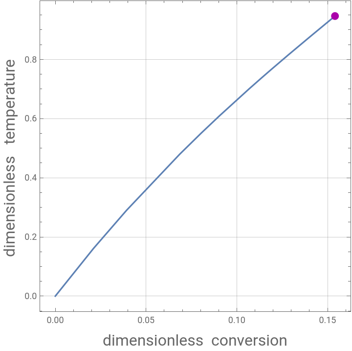
Steady State One appears as the Magenta dot on the Temperature and Conversion parametric plot
In[]:=
plt1=Show[ParametricPlot[Evaluate[{[t],[t]}/.sol[0,0]],{t,0,1000},FrameLabel{Style["dimensionless conversion",16],Style["dimensionless temperature ",16]},PlotRangeAll,AspectRatio1,FrameTrue,GridLinesAutomatic],Graphics[{Darker@Magenta,PointSize[0.025],Point[{a2,a1}/.root1]}]]
x
2
x
1
Out[]=
In[]:=
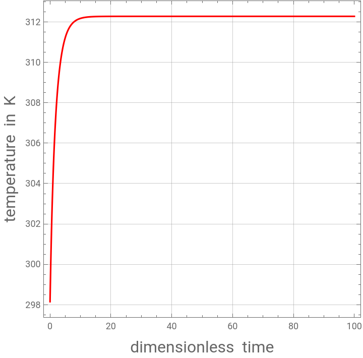
PLT1=Plot[Evaluate[298.15/19.9756[t]+298.15/.sol[0,0]],{t,0,100},FrameLabel{Style["dimensionless time",16],Style["temperature in K",16]},PlotRangeAll,PlotStyleRGBColor[1,0,0],AspectRatio1,FrameTrue,GridLinesAutomatic]
x
1
Out[]=
In[]:=
PLT2=Plot[Evaluate[[t]/.sol[0,0]],{t,0,100},PlotRangeAll,PlotStyleRGBColor[1,0,0],FrameLabel{Style["dimensionless time",16],Style["conversion ",16]},AspectRatio1,FrameTrue,GridLinesAutomatic]
x
2
Out[]=
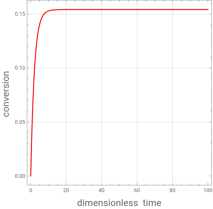
Steady state conversion
Steady state temperature in Kelvin
Steady State two appears as the Magenta dot on the Temperature and Conversion parametric plot
Steady state conversion
Steady state temperature in Kelvin
Showing both stable steady state temperature in the same plots
In[]:=
Show[PLT1,PLT3]
Showing both stable steady state conversion in the same plots
In[]:=
Show[PLT2,PLT4]
Phase plane plot. Steady state one, two and three are the red, green and blue dots respectively. One can see clearly that steady states one and two are stable (red and green dots) while steady state three is a saddle point (blue dot). Temperature overshoot is observed. Knowing about possible overshoot behavior is a valuable information since temperature overshoot can lead to safety problems.
In[]:=
tbl=Table[plt[i],{i,0,99,3}];
In[]:=
TBL=Table[PLT[i],{i,0,99,2}];
In[]:=
TbL=Table[plot[i],{i,0,99,4}];
In[]:=
Show[Flatten[Join[TBL,tbl,TbL]],Graphics[{{PointSize[0.02],RGBColor[1,0,0],Point[pt1]},{PointSize[0.02],
RGBColor[0,1,0],Point[pt2]},{PointSize[0.02],RGBColor[0,0,1],Point[pt3]}}],PlotRange->{{0,1},{0,6}},
FrameLabel{Style["dimensionless conversion",16],Style["dimensionless temperature ",16]},AspectRatio1,Frame True,GridLinesAutomatic]
RGBColor[0,1,0],Point[pt2]},{PointSize[0.02],RGBColor[0,0,1],Point[pt3]}}],PlotRange->{{0,1},{0,6}},
FrameLabel{Style["dimensionless conversion",16],Style["dimensionless temperature ",16]},AspectRatio1,Frame True,GridLinesAutomatic]
References
References
◼
[1] B. W. Bequette, Process Dynamics, Modeling, Analysis and Simulation, Englewood: Prentice Hall, 1998.
◼
[2] A. Varma and M. Morbidelli, Mathematical Methods in Chemical Engineering, Oxford: Oxford University Press, 1997.
CITE THIS NOTEBOOK
CITE THIS NOTEBOOK
Dynamic of a Diabatic Continuous Stirred Tank Reactor
by Housam Binous and Ahmed Bellagi
Wolfram Community, STAFF PICKS, February 10, 2024
https://community.wolfram.com/groups/-/m/t/3120241
by Housam Binous and Ahmed Bellagi
Wolfram Community, STAFF PICKS, February 10, 2024
https://community.wolfram.com/groups/-/m/t/3120241