ORIGINAL ARTICLE: Tal Einav, Yuehaw Khoo, and Amit Singer, Quantitatively Visualizing Bipartite Datasets, Phys. Rev. X 13, 021002. DOI: https://doi.org/10.1103/PhysRevX.13.021002
Article Abstract: As experiments continue to increase in size and scope, a fundamental challenge of subsequent analyses is to recast the wealth of information into an intuitive and readily interpretable form. Often, each measurement conveys only the relationship between a pair of entries, and it is difficult to integrate these local interactions across a dataset to form a cohesive global picture. The classic localization problem tackles this question, transforming local measurements into a global map that reveals the underlying structure of a system. Here, we examine the more challenging bipartite localization problem, where pairwise distances are available only for bipartite data comprising two classes of entries (such as antibody-virus interactions, drug-cell potency, or user-rating profiles). We modify previous algorithms to solve bipartite localization and examine how each method behaves in the presence of noise, outliers, and partially observed data. As a proof of concept, we apply these algorithms to antibody-virus neutralization measurements to create a basis set of antibody behaviors, formalize how potently inhibiting some viruses necessitates weakly inhibiting other viruses, and quantify how often combinations of antibodies exhibit degenerate behavior.
The following code reproduces the plots in the main text. Made on Mathematica version 13.2.0 for Windows.
Raw data can be found in the initialization section.
Further details can be found in attachments of this post.
Raw data can be found in the initialization section.
Further details can be found in attachments of this post.
Figures
Figures
Figure 1: Overview of MDS
Figure 1: Overview of MDS
We compare the classic localization problem (where distance can be measured between any pair of entries) with bipartite localization (where distance can only be measured between, and not within, two classes of entries).
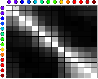
Panel A: Color-Color Distance
Panel A: Color-Color Distance
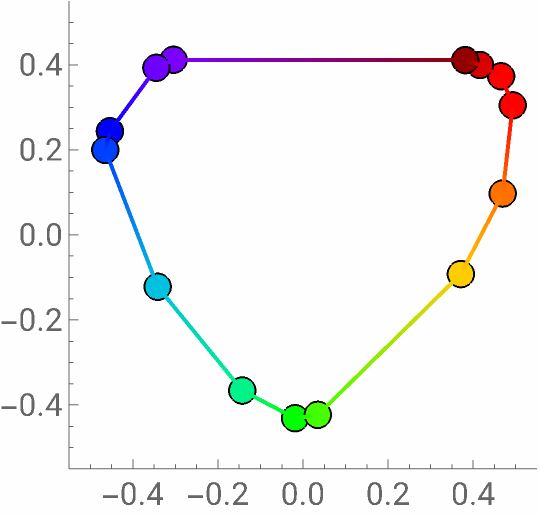
An example of classic localization using the canonical color wheel example. We apply metric MDS to previously published data.
In[]:=
(*Table4.1(page65)of
ModernMDS
byBorg&Groenen*)distRaw={{0},{0.86,0},{0.42,0.50,0},{0.42,0.44,0.81,0},{0.18,0.22,0.47,0.54,0},{0.06,0.09,0.17,0.25,0.61,0},{0.07,0.07,0.10,0.10,0.31,0.62,0},{0.04,0.07,0.08,0.09,0.26,0.45,0.73,0},{0.02,0.02,0.02,0.02,0.07,0.14,0.22,0.33,0},{0.07,0.04,0.01,0.01,0.02,0.08,0.14,0.19,0.58,0},{0.09,0.07,0.02,0.00,0.02,0.02,0.05,0.04,0.37,0.74,0},{0.12,0.11,0.01,0.01,0.01,0.02,0.02,0.03,0.27,0.50,0.76,0},{0.13,0.13,0.05,0.02,0.02,0.02,0.02,0.02,0.20,0.41,0.62,0.85,0},{0.16,0.14,0.03,0.04,0.00,0.01,0.00,0.02,0.23,0.28,0.55,0.68,0.76,0}};distMatrix=PadRight[#,Length@distRaw]&/@distRaw;distMatrix=distMatrix+Transpose@distMatrix+IdentityMatrix[Length@distMatrix];(*Transformfromdissimilaritytosimilarity*)distMatrix=1-distMatrix;In[]:=
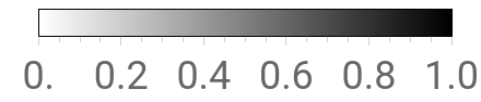
wavelengthsColors=ColorData["VisibleSpectrum"]/@{434,445,465,472,490,504,537,555,584,600,610,628,651,674};ArrayPlot[distMatrix,PlotRangePaddingNone,ImageSize->200,Frame->True,Mesh->True,MeshStyleDirective[Black,Thin],FrameTicks{MapIndexed[{First@#2,Row[{Graphics[{#,EdgeForm[Directive[Thickness[Small],Black]],Disk[]},ImageSize->9]}]}&,wavelengthsColors],None,None,MapIndexed[{First@#2,Row[{Graphics[{#,EdgeForm[Directive[Thickness[Small],Black]],Disk[]},ImageSize->9]}]}&,wavelengthsColors]},AspectRatio0.8,ColorFunctionScalingFalse]BarLegend[{GrayLevel[1-#]&,{0,1}},LegendLayout"Row",LabelStyle{FontSize18},FrameStyle->Directive[Thin,Black]]
Out[]=
Out[]=
coordsSDP=sdp[distMatrix];coordsSDP={0.04,0.1}+{-1,1}RotationTransform[2.78][#]&/@coordsSDP;plotColors=ListPlotList/@coordsSDP,Frame->{True,True,False,False},FrameTicksConstantArray,2,Axes->False,PlotMarkersplotMarker[0.065,"EdgeThickness"Medium],PlotStylewavelengthsColors,PlotRangeConstantArray[0.55{-1,1},2],AspectRatio1,ImageSize270,Epilog{Thick,Line[coordsSDP,VertexColorswavelengthsColors],Line[{coordsSDP[[-1]],coordsSDP[[1]]},VertexColorswavelengthsColors[[{-1,1}]]]},FrameTicksStyle16
Out[]=
Panel B: Schematic of Antibody-Virus Distance
Panel B: Schematic of Antibody-Virus Distance
Below we draw some schematic antibody-virus data to explain the benefits of embedding this bipartite data.
In[]:=
ArrayPlot,PlotRangePaddingNone,ImageSize->300,ColorFunctionScalingFalse,Frame->True,Mesh->True,MeshStyleDirective[Black,Thin],ColorRules{_Missing->colorMissing,val_Real:>GrayLevel[1-Rescale[val,MinMax@DeleteCases[Flatten@plotData,_Missing]]]},FrameTicks{MapIndexed[{First@#2,Row[{Graphics[{colorAbInMixture,markerAb["Thickness"0.01][[1,1]]},ImageSize->20]}]}&,Range@9],None,None,MapIndexed[{First@#2,Column[{Graphics[{#,markerVirus["Opacity"1,"OpacityFaceFormFactor"1][[1,1]]},ImageSize->22]},AlignmentCenter]}&,{,,,,,,,,,,,}]},AspectRatio0.8

Out[]=
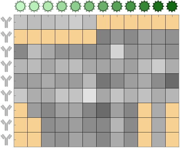
Note: The right panel in Figure 1b was only a schematic
Figure 2: Phase Diagram of Synthetic Data
Figure 2: Phase Diagram of Synthetic Data
Comparison of metric MDS, bipartite MDS, and SDP at different noise levels and fractions of missing values.
◼
For speed, the values for the phase diagrams are canned in the initialization section
In[]:=
methods={"mMDS","cMDS","SDP"};legPhaseDigrams=BarLegend[{ColorData["StarryNightColors"],{0,1}},LegendMarkerSize->200,Ticks->({#,If[MemberQ[Range[0,1,0.2],#],format[#,1],""]}&/@Range[0,1,0.1]),LabelStyle->14];legExamplePlots=PointLegend[ColorData[95]/@{1,2,1,2},font/@{"Virus (Ground Truth)","Virus (Numerical)","Antibody (Ground Truth)","Antibody (Numerical)"},LegendMarkers{plotMarker[0.05],plotMarker[0.7×0.05],plotMarker[1.125×0.05,"Type""Square"],plotMarker[0.7×1.125×0.05,"Type""Square"]},LegendFunctionframe];Grid[{Append[Riffle[Table[drawPhaseDiagram[dataPhaseDiagram,method,MaxPlotPoints25,InterpolationOrder1],{method,methods}],SpanFromLeft,{2,-1,2}],legPhaseDigrams],Append[Flatten[drawExamplePlots/@methods],legExamplePlots]},Spacings{2,2},Alignment{Left}]
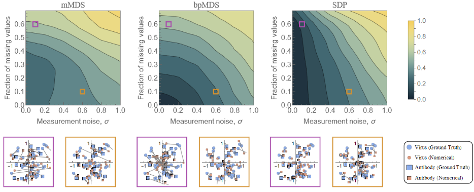
Figure 3: Outliers
Figure 3: Outliers
Analyzing how the embedding algorithms perform with several large outliers.
In[]:=
{nVirus,nAb}={10,12};outliers={{1,1},{2,2},{3,1}}->10;lowerBounds={{6,8},{2,7},{9,5},{8,5},{7,7},{8,6},{6,2},{7,10},{4,2},{4,9},{5,3},{6,9},{1,2},{8,1},{9,8},{7,12},{4,5},{9,11}};upperBounds={{8,11},{8,4},{3,9},{4,10},{4,8},{9,9},{7,3},{8,7},{2,1},{4,12},{1,6},{6,5},{2,3},{3,5},{10,1},{1,10},{10,8},{5,7}};plotMarkerSize=12;
In[]:=
{coords,distMatrix}=exampleData[{nVirus,nAb},0.];distMatrixOutliers=ReplacePart[distMatrix,outliers];(*Showdistancematrixcorruptedwithlargeoutliers*){showVirusCoords,showAbCoords,showDistMatrixOutliers}={showGrid[List/@Prepend[font@Row[{"(",format[#[[1]],2],",",format[#[[2]],2],")"}]&/@First@coords,""]],showGrid[List/@Prepend[font@Row[{"(",format[#[[1]],2],",",format[#[[2]],2],")"}]&/@Last@coords,""]],MatrixForm[MapAt[Item[#->font[Last@outliers,Bold,Darker@Red],BackgroundLightRed]&,Map[font@format[#,2]&,distMatrix,{2}],First@outliers]]};(*cMDSandSDPonoutlierdata*){resSDP,resClassicalMDS,resMetricMDS}=Quiet@coordsMDS=sdp[distMatrixOutliers];ShowanalyzeMDS[coords,coordsMDS,LegendLabel->"SDP","AddToPlotLabel"->Row[{Style["SNL-SDP",Bold],", "}],"PlotLabelSize"->15,"ShowLegend"->False,"ConnectNumericToActual"True,"Comparing""Distance","PenalizeError""RMSE","ErrorLabel""RMSE",PlotRange->1.1{-1,1},PlotStyle->colorsEmbedding,"PlotMarkerSize"->plotMarkerSize],Ticks->ConstantArray,2,coordsMDS=classicalMDS[distMatrixOutliers];analyzeMDS[coords,coordsMDS,"AddToPlotLabel"->Row[{Style["BP-cMDS",Bold],", "}],"PlotLabelSize"->15,"ShowLegend"->False,"ConnectNumericToActual"True,"Comparing""Distance","PenalizeError""RMSE","ErrorLabel""RMSE",PlotStyle->colorsEmbedding,"PlotMarkerSize"->plotMarkerSize],coordsMDS=metricMDS[distMatrixOutliers,"SearchMethod"Automatic,"SearchPoints"Automatic,"Comparing""Distance","PenalizeError""MeanSquaredError"];analyzeMDS[coords,coordsMDS,LegendLabel->"mMDS","AddToPlotLabel"->Row[{Style["mMDS",Bold],", "}],"PlotLabelSize"->15,"ConnectNumericToActual"True,"Comparing""Distance","PenalizeError""RMSE","ErrorLabel""RMSE",PlotStyle->colorsEmbedding,"ShowLegend"->False,"PlotMarkerSize"->plotMarkerSize];gridOutliers=Grid[{{Grid[{{showVirusCoords,showAbCoords,Labeled[showDistMatrixOutliers,showGrid[{{"True Distance Matrix Corrupted Matrix D with Large Outliers"}}],Top]}},Spacings2,AlignmentTop],SpanFromLeft},{resMetricMDS,resClassicalMDS,resSDP}},Spacings{2,2}]
*
X
*
Y
*
D
Embedding data that contains upper and lower bounds
Figure 4: Antibody-Virus Data
Figure 4: Antibody-Virus Data
Here, we assess the embedding algorithms using antibody-virus neutralization data from Creanga 2021, with the raw data provided in the initialization section.
Visualizing the Ab-Virus Data
Visualizing the Ab-Virus Data
mMDS Solution
mMDS Solution
Using metric multidimensional scaling to embed this system into 2D. As described in Figure S3, we remove the five worst viruses and five worst antibodies whose positions cannot be robustly determined.
Leave-Some-Out Analysis - Embedding
Leave-Some-Out Analysis - Embedding
Comparing embeddings in 1D-4D for the three embedding algorithms. The results are canned for speed.
Showing leave-one-out results (tenfold cross-validation) for 2D embeddings.
Figure 5: Degeneracy of the Antibody Response
Figure 5: Degeneracy of the Antibody Response
Given the basis set of monoclonal antibody behaviors established by the embedding in Figure 4B, we explore when an antibody mixture exhibits a neutralization profile that cannot be closely replicated by an individual antibody.
Examples of 2-Antibody and 4-Antibody Mixtures
Examples of 2-Antibody and 4-Antibody Mixtures
Degeneracy for n-Antibody Mixtures
Degeneracy for n-Antibody Mixtures
Exploring the general case of random n-antibody mixtures, although we restrict the antibodies to lie within rectangles around the H1N1 and H3N2 virus subtypes (since antibodies further away represent the uninteresting case of weak antibodies that do not change the neutralization profile).
CITE THIS NOTEBOOK
CITE THIS NOTEBOOK
Quantitatively Visualizing Bipartite Datasets
by Tal Einav, Yuehaw Khoo, and Amit Singer
Wolfram Community, STAFF PICKS, September 20, 2023
https://community.wolfram.com/groups/-/m/t/3016918
by Tal Einav, Yuehaw Khoo, and Amit Singer
Wolfram Community, STAFF PICKS, September 20, 2023
https://community.wolfram.com/groups/-/m/t/3016918