The detection range and recognition performance of electro-optical systems are dependent on the incoherent optical Modulation Transfer Function (MTF) which is defined as the autocorrelation of the entrance pupil function. Analytical MTF calculations are often difficult because integration limits change with the autocorrelation variable and the calculation of those limits require detailed calculations. Here we show how to use the Boole function to calculate the autocorrelation of an arbitrary area, which enables the calculation of incoherent optical MTF for a wide variety of entrance pupil functions. These computations belongs to Chapter 4 of the book. Citation (original book): Ronald G. Driggers, Melvin H. Friedman, John W. Devitt, Orges Furxhi, Anjali Singh (2022), Introduction to Infrared and Electro-Optical Systems, Third Edition, Artech House, ISBN: 9781630818326. https://us.artechhouse.com/Introduction-to-Infrared-and-Electro-Optical-Systems-Third-Edition-P2271.aspx
Amazon: https://a.co/d/ghlvrj1
The book is Joseph W. Goodman Book Writing Award winner.
Amazon: https://a.co/d/ghlvrj1
The book is Joseph W. Goodman Book Writing Award winner.
0. Book Introduction
0. Book Introduction
This newly revised and updated edition offers a current and complete introduction to the analysis and design of Electro-Optical (EO) imaging systems. The Third Edition provides numerous updates and several new chapters including those covering Pilotage, Infrared Search and Track, and Simplified Target Acquisition Model.
The principles and components of the Linear Shift-Invariant (LSI) infrared and electro-optical systems are detailed in full and help you to combine this approach with calculus and domain transformations to achieve a successful imaging system analysis. Ultimately, the steps described in this book lead to results in quantitative characterizations of performance metrics such as modulation transfer functions, minimum resolvable temperature difference, minimum resolvable contrast, and probability of object discrimination.
The book includes an introduction to two-dimensional functions and mathematics which can be used to describe image transfer characteristics and imaging system components. You also learn diffraction concepts of coherent and incoherent imaging systems which show you the fundamental limits of their performance. By using the evaluation procedures contained in this desktop reference, you become capable of predicting both sensor test and field performance and quantifying the effects of component variations. The book contains over 800 time-saving equations and includes numerous analyses and designs throughout. It also includes a reference link to special website prepared by the authors that augments the book in the classroom and serves as an additional resource for practicing engineers.
With its comprehensive coverage and practical approach, this is a strong resource for engineers needing a bench reference for sensor and basic scenario performance calculations. Numerous analyses and designs are given throughout the text. It is also an excellent text for upper-level students with an interest in electronic imaging systems.
1. Theory
1. Theory
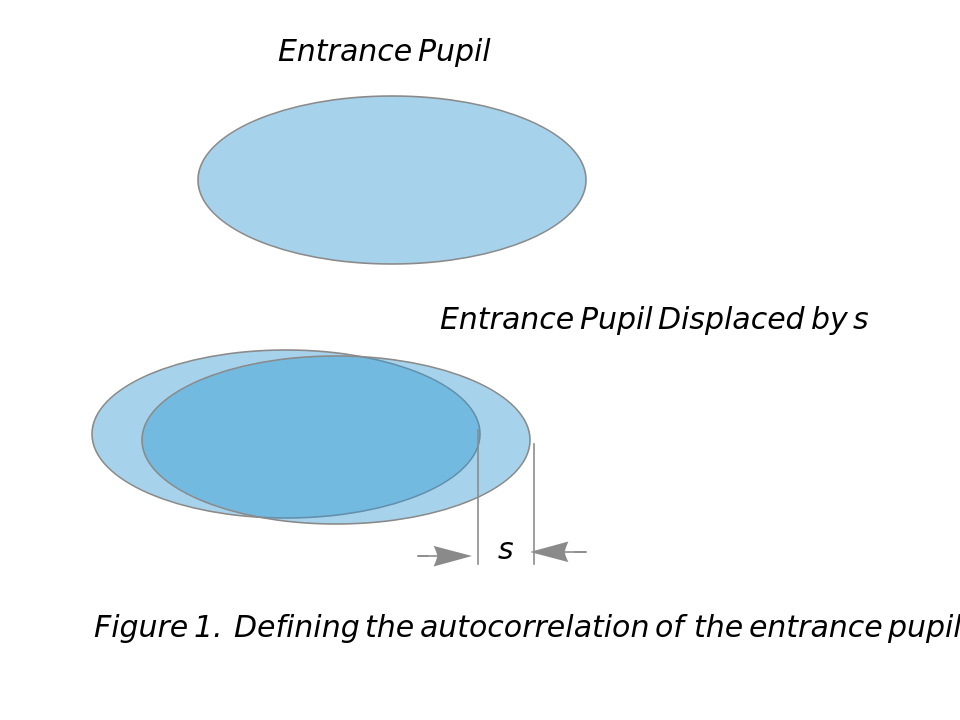
Figure 1, which was drawn using Mathematica’s drawing tools, defines the autocorrelation of the entrance pupil. The entrance pupil is shown at the top of the figure. The entrance pupil and the entry pupil displaced by a distance to the right is shown at the bottom of the figure. The region of overlap is the darker blue region in Figure 1. Clearly the area of overlap depends on . The incoherent optical MTF is commonly expressed as a spatial frequency either in cycles/mm or in cycles/mr as given by (1a) and (1b)
s
A
OL
s
(1a) (1b) where spatial frequency is in cycles/mrwhere is the area of the entrance pupil, λ is the average wavelength of the optical radiation in units of micrometers and fl is the focal length of the lens in mm. In (1)a the factor allows the frequency to be in cycles/mm when the units of s and fl are mm and the units of λ are micrometers.
MTF(f)=(s)wherespatialfrequencyfisincycles/mm
A
OL
A
0
sλflf
-3
10
MTF(f)=(s
A
OL
A
0
sλf
f
A
0
-3
10
f
Although Figure 1 shows the displacement in the positive x-direction the displacement could just as well have been taken in the y-direction or in any intermediate direction. When is taken in the x-direction the frequency in (1a) or (1b) is a frequency in the x-direction and is denoted by ; when is taken in the y-direction the frequency in (1a) or (1b) is denoted by .
s
s
f
x
s
f
y
The calculation of (s) can be difficult to do analytically by hand for two reasons: 1) For obscured apertures the integral limits change with and the size of the obscuration; 2) Even when the limits are known the integrals are sometimes difficult to evaluate analytically. A strength of Mathematica is that it allows (s) to be calculated without the user having to explicitly specify integration limits. As shown below this is done in Mathematica using defined functions Boole and Integrate.
A
OL
s
A
OL
The above equations are useful if the MTF is to be expressed in cycles/mm or cycles/mr. Sometimes it is convenient to express the MTF in a normalized frequency . As increases, for all larger than the overlap area is zero. Typically the value in the x-direction is different from the value in the y-direction. An optical cutoff frequency in the and directions are defined in terms of .
f
n
s
s
s
max
A
0
s
max
s
max
f
oco
x
y
s
max
(2a) =[cycles/mr](2b) =λfl[cycles/mm]In (2a) and (2b) and fl are expressed in mm and the wavelength λ is expressed in micrometers. The dimensionless normalized frequency is defined by(3) =
f
oco
s
max
λ
f
oco
s
max
-3
10
s
max
f
n
f
n
f
f
oco
2. Code
2. Code
Codes are given below corresponding to the binary choices: MTF given in the vertical or horizontal directions, analytical/numerical result, frequency given in normalized units, cycles per mm and cycles per mr.
The user defined Mathematica functions MTFNoramilzedEqHor and MTFNormalizedEqVer given below enable computer calculation of analytical MTF functions. An important argument of these functions is the inequality that defines the entrance pupil. To have these functions properly output a normalized frequency the entrance pupil shape should satisfy the following rules:
1. The entrance pupil shape is input in units of mm.
2. When using MTFNoramilzedEqHor the entrance pupil shape is normalized so that is one in the horizontal direction.
3. When using MTFNoramilzedEqVer the entrance pupil shape is normalized so that is one in the vertical direction.
2. When using MTFNoramilzedEqHor the entrance pupil shape is normalized so that
s
max
3. When using MTFNoramilzedEqVer the entrance pupil shape is normalized so that
s
max
MTFNormalizedEqHor outputs an MTF equation in units of normalized frequency with the entrance pupil shape defined by Ineq. Here {x,y} corresponds to the variables used in Ineq. Similar comments apply in MTFNormalizedEqVer.
f
In[]:=
MTFNormalizedEqHor[Ineq_,{x_,y_},f_]:=Module{temp,A0,s},A0=Integrate[Boole[Ineq],{x,-∞,∞},{y,-∞,∞}];temp=Integrate[Boole[Ineq&&(Ineq/.x(x-s))],{x,-∞,∞},{y,-∞,∞},Assumptionss≥0];temp/.sf
1
A0
In[]:=
MTFNormalizedEqVer[Ineq_,{x_,y_},f_]:=Module{temp,A0,s},A0=Integrate[Boole[Ineq],{x,-∞,∞},{y,-∞,∞}];temp=Integrate[Boole[Ineq&&(Ineq/.y(y-s))],{x,-∞,∞},{y,-∞,∞},Assumptionss≥0];temp/.sf
1
A0
NMTFNormalizedHor outputs NPoints which numerically describe the normalized MTF. The entrance pupil shape is described by Ineq and {x,y} corresponds to the variables used in Ineq. Similar comments apply to NMTFNormalizedVer.
In[]:=
NMTFNormalizedHor[Ineq_,{x_,y_},NPoints_]:=Module{A0,s},A0=NIntegrate[Boole[Ineq],{x,-∞,∞},{y,-∞,∞}];Tables,NIntegrate[Boole[Ineq&&(Ineq/.x(x-s))],{x,-∞,∞},{y,-∞,∞}],s,0,1,//Chop
1
A0
1
NPoints
In[]:=
NMTFNormalizedVer[Ineq_,{x_,y_},NPoints_]:=Module{A0,s},A0=NIntegrate[Boole[Ineq],{x,-∞,∞},{y,-∞,∞}];Tables,NIntegrate[Boole[Ineq&&(Ineq/.y(y-s))],{x,-∞,∞},{y,-∞,∞}],s,0,1,//Chop
1
A0
1
NPoints
MTFCyclesPerMmEqHor produces an equation that describes the horizontal MTF in units of cycles per mm. The inputs are an inequality Ineq that describes the entrance pupil shape, {x,y} the variables used in the inequality, the wavelength λ and the focal length fl. The variable used to describe frequency in the equation is f. Similar comments apply to MTFCyclesPerMmEqVer.
In[]:=
MTFCyclesPerMmEqHor[Ineq_,{x_,y_},λ_,fl_,f_]:=Module{temp,A0,s},A0=Integrate[Boole[Ineq],{x,-∞,∞},{y,-∞,∞}];temp=Integrate[Boole[Ineq&&(Ineq/.x(x-s))],{x,-∞,∞},{y,-∞,∞},Assumptionss≥0];(*sisinmm,λisinμ,flisfocallengthinmm,fisincyclesmm,Facotrofchangesμtomm*)temp/.sλflf
1
A0
-3
10
-3
10
In[]:=
MTFCyclesPerMmEqVer[Ineq_,{x_,y_},λ_,fl_,f_]:=Module{temp,A0,s},A0=Integrate[Boole[Ineq],{x,-∞,∞},{y,-∞,∞}];temp=Integrate[Boole[Ineq&&(Ineq/.y(y-s))],{x,-∞,∞},{y,-∞,∞},Assumptionss≥0];(*sisinmm,λisinμ,flisfocallengthinmm,fisincyclesmm,Facotrofchangesμtomm*)temp/.sλflf
1
A0
-3
10
-3
10
NMTFCyclesPerMmHor outputs a table with NPoints that numerically describes the horizontal MTF. The entrance pupil shape is described by Ineq that utilizes variables {x,y}. The wavelength of the incident radiation, focal length of the optical system and the maximum displacement that corresponds to the cutoff frequency are given by λ, fl and smax . Similar comments apply to NMTFCyclesPerMmVer.
In[]:=
NMTFCyclesPerMmHor[Ineq_,{x_,y_},λ_,fl_,smax_,NPoints_]:=Module{temp,A0,s},A0=NIntegrate[Boole[Ineq],{x,-∞,∞},{y,-∞,∞}];temp=Tables,NIntegrate[Boole[Ineq&&(Ineq/.x(x-s))],{x,-∞,∞},{y,-∞,∞}],s,0,smax,//Chop;(*sisinmm,λisinμ,flisfocallengthinmm,fisincyclesmm,factorofchangesμtomm*)temp/.{a_,b_}λfl,b
1
A0
smax
NPoints
-3
10
a
-3
10
In[]:=
NMTFCyclesPerMmVer[Ineq_,{x_,y_},λ_,fl_,smax_,NPoints_]:=Module{temp,A0,s},A0=NIntegrate[Boole[Ineq],{x,-∞,∞},{y,-∞,∞}];temp=Tables,NIntegrate[Boole[Ineq&&(Ineq/.y(y-s))],{x,-∞,∞},{y,-∞,∞}],s,0,smax,//Chop;(*sisinmm,λisinμ,flisfocallengthinmm,fisincyclesmm,factorofchangesμtomm*)temp/.{a_,b_}λfl,b
1
A0
smax
NPoints
-3
10
a
-3
10
MTFCyclesPerMrHor produces an equation that describes the horizontal MTF in units of cycles per mr. The entrance pupil shape is described by an inequality Ineq that utilizes variables {x,y}. The incident radiation has wavelength λ. The symbol f is used for frequency in the output equation. Similar comments apply to MTFCyclesPerMrVer.
In[]:=
MTFCyclesPerMrEqHor[Ineq_,{x_,y_},λ_,f_]:=Module{temp,A0,s},A0=NIntegrate[Boole[Ineq],{x,-∞,∞},{y,-∞,∞}];temp=Integrate[Boole[Ineq&&(Ineq/.x(x-s))],{x,-∞,∞},{y,-∞,∞},Assumptionss≥0];(*sisinmm,λisinμ,fisincycles/mm*)temp/.sλf
1
A0
NMTFCyclesPerMrHor outputs a table with NPoints that describes the horizontal MTF in cycles per mr. The entrance pupil shape is described by an inequality Ineq that utilizes variables {x,y}. The incident radiation has wavelength λ and smax is the displacement that corresponds to the cutoff frequency. Similar comments apply to NMTFCyclesPerMrVer.
3. Examples
3. Examples
This section uses several examples to illustrate the use of code given in Section 2.
Circular Entrance Pupil
Circular Entrance Pupil
Figure 2 was drawn using Mathematica’s drawing tools. It could have been drawn using RegionPlot.
Square Entrance Pupil
Square Entrance Pupil
Semi-Circular Aperture
Semi-Circular Aperture
Equations in Section 3 demonstrate that Mathematica reproduces known results.
4. Verification
4. Verification
This section uses several examples to illustrate the use of code given in Section 2 and to validate results produced by that code.
Circular Entrance Pupil
Circular Entrance Pupil
Equation 4 is a well-known expression. Evidence that NMTFNormalizedHor is correct is obtained by comparing the output of
with (4).
Figure 5. Comparison of numerical and analytical calculations for circular entrance pupil .
Square Entrance Pupil
Square Entrance Pupil
Equation 5 is a well-known expression. Gain additional evidence NMTFNormalizedHor is correct by comparing its output with the results of (5).
Figure 6. Comparison of numerical and analytical calculations for a square entrance pupil
Semi-circular aperture
Semi-circular aperture
Use NMTFNormalizedHor to gain confidence in this function and MTFNOrmalizedEqHor by determining if they are consistent. The command used to generate numerical results is
Figure 7. Comparison of numerical and analytical calculations for a semi-circular entrance pupil.
Elliptical Entrance Pupil
Elliptical Entrance Pupil
Figure 8 was constructed using Mathematica’s drawing tools. The entrance pupil shape is shown more accurately using RegionPlot.
Calculate the MTF in the horizontal and vertical directions for the entrance pupil illustrated in Fig. 8 for the case where the average wavelength of the incident radiation is 10 μ and the focal length is 10 mm.
Exhibit the equation and numerical MTF results in the horizontal direction
Graph the equation for the MTF in the horizontal direction and compare with numerical results
Figure 9a.Comparison of numerical and analytical horizontal MTF calculations for entrance pupil of Fig.8.
Graph the equation for the MTF in the vertical direction and compare with numerical results
Figure 9b.Comparison of numerical and analytical vertical MTF calculations for entrance pupil of Fig .8.
Distributed Entrance Pupil
Distributed Entrance Pupil
Figure 10 was constructed using Mathematica’s drawing tools and Paint. In Fig. 10 the center-to-center distance in the vertical and horizontal directions is 3.8 mm and each of the four clear areas has a diameter of 1.2 mm.
By symmetry, the MTF in the vertical and horizontal directions are the same. Commands used to define the distributed aperture, RegionEntiree, are given below.
The shape of the distributed pupil is shown more accurately using RegionPlot
Commands used to generate the equation and table that define the horizontal or vertical MTF are given below for the case where λ=10 μ and fl=10 mm
Exhibit temp1 and temp2
The equation stored in temp1 is an original result. Graph the MTF in the horizontal or vertical direction for the distributed aperture shown in Fig. 10
Figure 11. Analytical and numerical calculation of horizontal or vertical MTF of the aperture shown in Figure 10.
Racetrack Aperture
Racetrack Aperture
The racetrack aperture is defined by RegionEntire and is graphed using RegionPlot.
Figure 12 was drawn by pasting the above RegionPlot into Paint, inserting the dimensions and lines using paint and the arrows using Mathematica.
In Fig. 12 a clear circular entrance pupil 5.0 mm in diameter is truncated to be 3.4 mm in the vertical direction. The following commands output the equations and numerical tables for the horizontal and vertical MTF for a system with an average wavelength of 10 μ and a focal length of 10 mm.
Exhibit the MTF equation and numerical data which describes the horizontal MTF for the racetrack aperture shown in Fig. 12 and graph the data
Similarly, the vertical racetrack MTF is displayed
5. Summary and Conclusions
5. Summary and Conclusions
In this paper, functions have been written in Mathematica that take as input the shape and size of the entrance pupil and output either analytically or numerically incoherent optical MTF functions. Although CODEV, ZEMAX and other programs can numerically calculate these incoherent optical MTFs I am not aware of any other program that can take as input an analytical expression of the input pupil and output an analytical MTF in the specified direction. If an exact description of the entrance pupil is input, then code exhibited here that produces analytical results output an exact expression for the MTF in the specified direction.
Functions exhibited here has been verified with several entrance pupil shapes by comparing Mathematica generated analytical and numerical expressions against themselves and with numerical calculations done by CODEV.
For a sufficiently complicated entrance pupil description, functions exhibited here that produce an analytical result may grind on endlessly and fail to produce an analytical result. For an entrance pupil that has sufficiently fine detail, functions exhibited here that produce a numerical result may need tweaking to properly reflect changes in the MTF caused by fine detail.
This notebook demonstrates computer programs that programs that produce analytical MTF results for cases where it is either too hard or too tedious to get analytical results by hand calculations. This notebook can serve as a user’s manual for the functions given in Section 2.
CITE THIS NOTEBOOK
CITE THIS NOTEBOOK
Introduction to infrared and electro-optical systems
by Ronald G. Driggers, Melvin H. Friedman, John W. Devitt, Orges Furxhi, Anjali Singh
Wolfram Community, STAFF PICKS, February 2, 2021
https://community.wolfram.com/groups/-/m/t/2182449
by Ronald G. Driggers, Melvin H. Friedman, John W. Devitt, Orges Furxhi, Anjali Singh
Wolfram Community, STAFF PICKS, February 2, 2021
https://community.wolfram.com/groups/-/m/t/2182449