The aim of the project is to investigate the statistical features of over-dimension fields in a cosmological setting. The over-dimension field of a graph is defined as the excess Hausdorff dimension computed at each vertex with respect to the global average. The two-point correlation function has become one of the most popular statistical tools in cosmology. We build an estimator in a graph-based framework, and apply it to over-dimension fields. First, this is done by considering graphs generated from sprinkling of known geometries. The impact of using coordinates or geodesics to compute vertex separation is addressed and the formalism is then extended to higher order statistics (relevant for non-gaussian fields). We apply this approach to GRAVITAS-generated hypergraphs with an underlying FLRW metric in which some local dimension perturbation is introduced, and the main resulting features are discussed. This is relevant to the construction of observational predictions in the context of the Wolfram Physics Project, and potentially to the prediction of signatures in the Large-Scale Structure of the Universe and on the Cosmological Stochastic Gravitational-Wave Background anisotropies.
Introduction
Introduction
The Wolfram model for discretized spacetime is a novel approach that considers our universe to be made up of discrete connections rather than continuous variables. This model utilizes hypergraphs, which are generalizations of graphs that allow an edge to connect any number of nodes, to represent the structure of space. Space is represented by a hypergraph and the dynamics are determined by abstract replacement operations on set systems. The conformal structure of spacetime is represented by a causal graph. This model also introduces a discrete notion of Riemann and Ricci curvature for hypergraphs. In terms of practical computation, the Wolfram model seems to be more efficient at generating results than numerical relativity, making it a promising method for practical computations in general relativity. In the model, space doesn’t inherently have any particular dimension. Instead, dimension is an emergent feature of the hypergraph and can vary with position and time. The Wolfram model posits that the universe started as infinite-dimensional and gradually cooled to become three-dimensional. Traditional general relativity describes spacetime in terms of a continuous manifold, which limits the phenomena it can describe. However, the underlying discreteness and variable dimension of space, allows for new exotic phenomena like dimension fluctuations in our universe, which are the main focus of this work. In order to study such dimension variability, we make use of a classical statistical tool in cosmology - the 2-point correlation function - to study the clustering and distribution of our dimension estimator across peculiar spatial manifolds and its evolution in time.
2-point Correlation Function
2-point Correlation Function
The 2-point correlation function, is a fundamental concept in statistical physics and cosmology. It quantifies the statistical relationship between pairs of points in a system or distribution. In essence, it measures the excess probability of finding two points at a certain separation compared to a random distribution . The 2 - point correlation function provides valuable information about the spatial distribution, clustering, and overall structure of objects or particles in a given system. It is widely used in various fields, including condensed matter physics, astrophysics, and cosmology, to study phenomena such as phase transitions, large - scale structure formation, and galaxy clustering.
For a generic field ρ, we are interested in analyzing its structure. One can then study deviations from the overall average. We then introduce a quantity δ (over-density field in cosmological context), so that δ(x)=(ρ(x)-<ρ>)/<ρ>.
The correlation function is then defined as ξ(x1,x2)=<δ(x1)δ(x2)>, where the field is computed at vector position x1 and x2.
One can also construct some further summary statistics by considering the correlation ξ(r) just as a function of separation r=|x2-x1|, or separation and angle θ with respect to a fixed line of sight, ξ(r,θ). The former would include all the information on the dataset for isotropic fields, but it can still be used as a probe to distill interesting features from the distribution.
Wolfram-Hausdorff Dimension
Wolfram-Hausdorff Dimension
The Wolfram-Hausdorff dimension is determined by identifying the dominant exponent in the volume expansion of a finite geodesic ball within the graph. This computation is a discrete counterpart to the standard Hausdorff dimension of a metric-measure space. The Wolfram-Hausdorff dimension provides one possible approach to define the discrete dimension for any graph, achieved by discretizing the power series expansion of a continuous Riemannian volume element. Note that this approach differs from alternative definitions like the Myrheim-Meyer dimension estimator, which relies on random sampling.
In practice, the Wolfram-Hausdorff dimension is evaluated at each vertex of a given graph by taking an average over geodesic balls of all radii up to the dimension of the graph itself. The average is weighted by a set of radial-dependent exponential factors, so that lower radii are more relevant in the evaluation. This allows to slightly contain boundary effects - note that for vertices near the borders the computation is biased - still preserving the overall information content.
This is then treated as a point-sampled field one can statistically analyze.
Since we are interested in the structure of the dimension distribution, we introduce the over-dimension as the reference quantity for our analysis. This is defined by computing the deviation of the Wolfram-Hausdorff dimension computed at each vertex with the overall average. In practice, it is implemented as
In[]:=
wavg[graph_,dim_,cont_]:=dims=ResourceFunction["WolframHausdorffDimension"][IndexGraph[graph],cont,Floor[dim],"Dimension","DimensionMethod"->Identity];Total[Table[dims[[i]]*Exp[-],{i,1,Floor[dim]}]]Total[Exp[-]&/@Range[Floor[dim]]];
2
(i/Floor[dim])
2
(#/Floor[dim])
[graph is a graph object, dim its size and cont the vertex in which the dimension is computed]
Build the Intuition : Main Function and Reference Tests
Build the Intuition : Main Function and Reference Tests
The main computation for the 2-point correlation function is splitted in sub-functions for easier storing and post-processing of the data.
CorrTuples computes the over-dimension for each vertex of the graph, generates all pairs of vertices, computes the separation and angle with respect to a fixed line of sight (in a effective “flat-sky approximation”) and groups them in a single dataset. binplot and binplot2d then generate the actual correlation visualization. They linearly bin the data in terms of their angle and separation, compute the over-dimension product and average over all the pairs within a single bin.
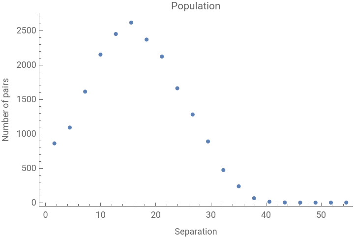
The function also provides a population array to assess how the data is distributed over different bins, in order to provide consistency checks and test the robustness of the chosen binning sizes.
Notice also that the notion of separation in a graph is different by the direct euclidian distance between two points. The code computes separation as the minimum-length edge path between two vertices.
Code
Code
Reference cases
Reference cases
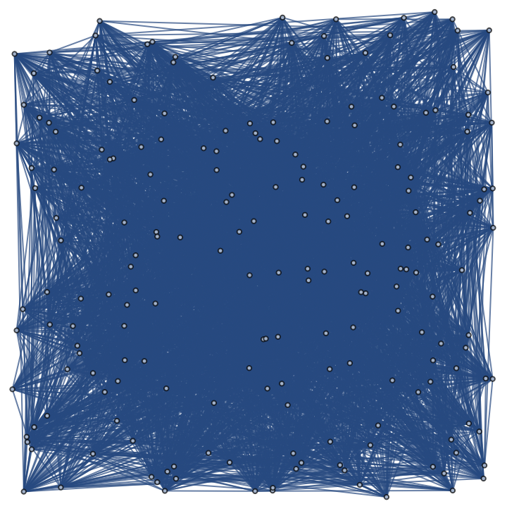
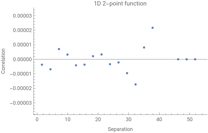
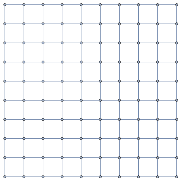
As reference examples, one may explore the correlation of regular grid graphs and totally random-distributed graphs. Intuitively, the former has same dimension at each point, providing an effective null over-dimension, while the latter should not show any structure since the spatial distribution of points is totally random and for high connectivity the local dimension does not show high variability. Thus, both cases should present no correlation signal and this is indeed what one retrieves when computing the 1D 2-point function. Notice that some boundary effects are still present. Notice also how the number of points per bin lowers for increasing separation, resulting in a less precise measurement.
The random case is particularly interesting, as it clearly shows the underlying geometrical interpretation. The vertices are randomly scattered implying no spatial correlation. The high connectivity of the graph also reduces the over-dimension magnitude resulting in an effective zero signal, with fluctuations due to the finite sampling.
The random case is particularly interesting, as it clearly shows the underlying geometrical interpretation. The vertices are randomly scattered implying no spatial correlation. The high connectivity of the graph also reduces the over-dimension magnitude resulting in an effective zero signal, with fluctuations due to the finite sampling.
In[]:=
dim=20;npoints=200;connectivity=0.2;originalGraph=GridGraph[{dim,dim}];edgeList=RandomGraph[BernoulliGraphDistribution[npoints,connectivity]];randomCoordinates=Association[Table[i->RandomReal[{1,dim},2],{i,VertexCount[originalGraph]}]];points=Graph[edgeList,VertexCoordinates->randomCoordinates];pardb=CorrTuples[points,dim];{points,binplot[pardb[[1]],pardb[[2]],20]}dim=10;points=GridGraph[{dim,dim}];pardb=CorrTuples[points,dim];{points,binplot[pardb[[1]],pardb[[2]],10]}
Out[]=
,
,
Out[]=
,
,
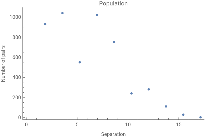
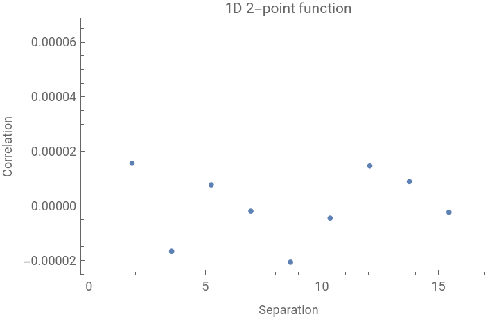
Over-Dimension Fields
Over-Dimension Fields
We now apply this formalism in a general-relativistic context, analyzing the over-dimension correlation function over discretized spatial hypersurfaces of known metrics. We make use of the GRAVITAS framework, which is a hypergraph-based numerical relativity code that utilizes unstructured adaptive mesh refinement. It incorporates various features such as the ability to perform the canonical 3 + 1 metric decomposition, compute evolution equations, constraint equations, and gauge satisfaction equations. These functionalities are achieved through components like ADMDecomposition. Additionally, Gravitas employs adaptive hypergraph methods like DiscreteHypersurfaceDecomposition to discretize the resulting evolution. It enables the coupling of arbitrary spacetimes with arbitrary matter/stress-energy distributions. The code is capable of solving the Einstein field equations both numerically and analytically. Furthermore, Gravitas provides an extensive library of built-in metrics, geometries, gauge choices, and coordinate systems.
Code
Code
Visualization Code
Visualization Code
Visualization
Visualization
Since the code is expensive to run, we directly report the final plots. The results can be retrieved from the attached .wxf files.
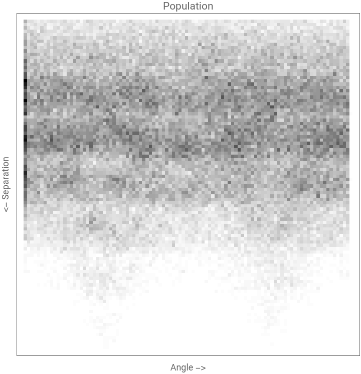
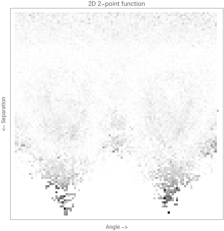
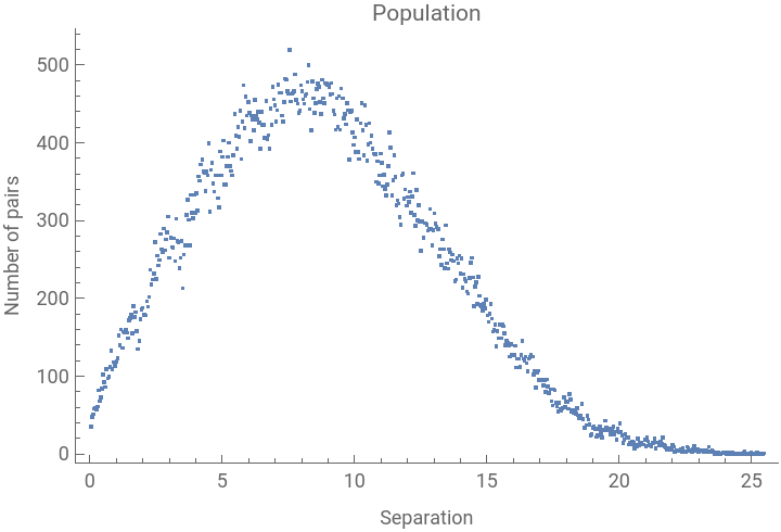
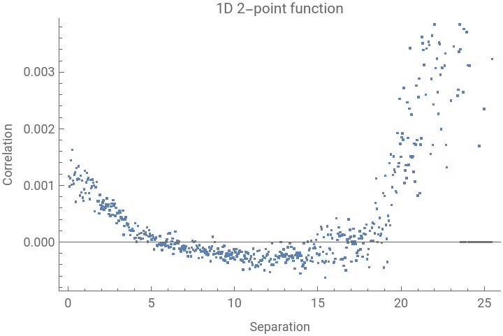
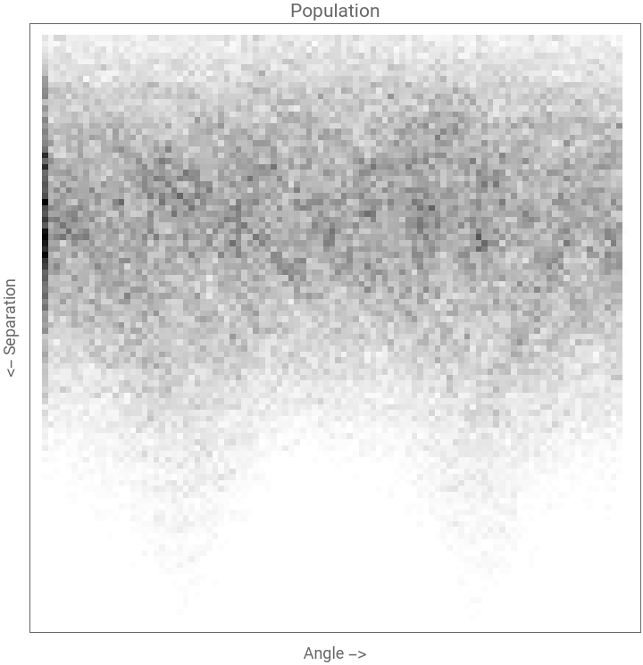
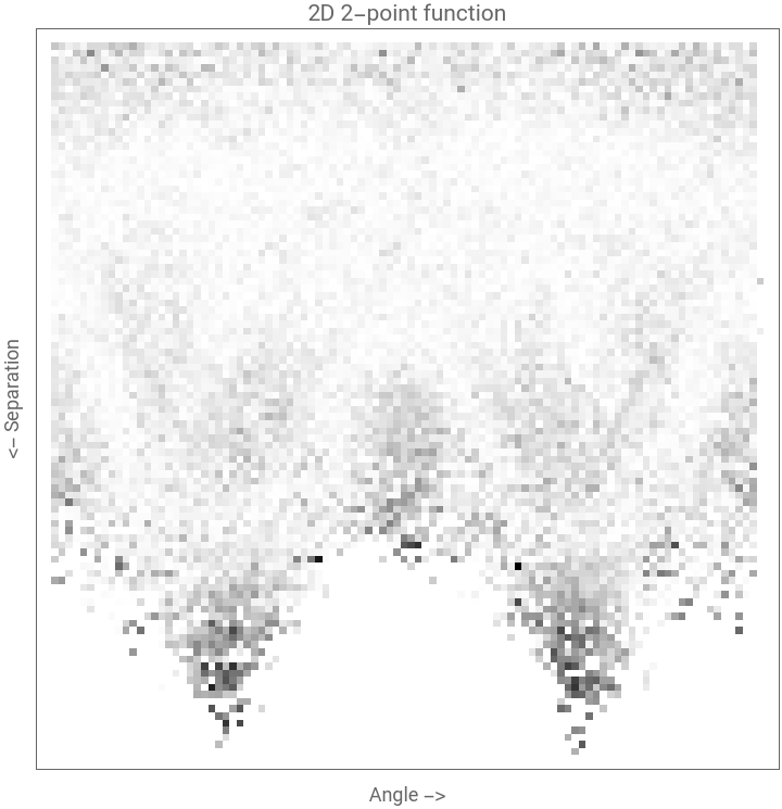
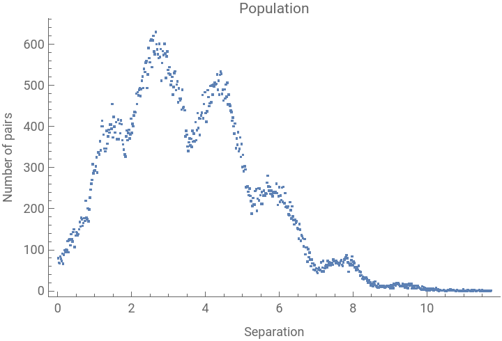
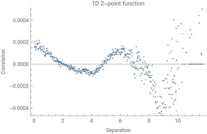
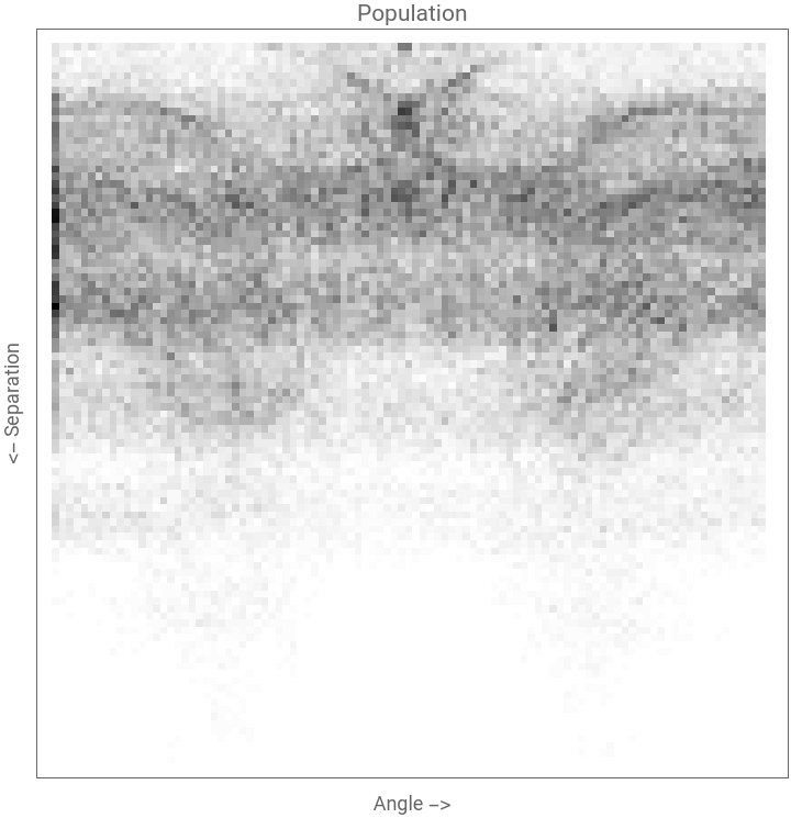
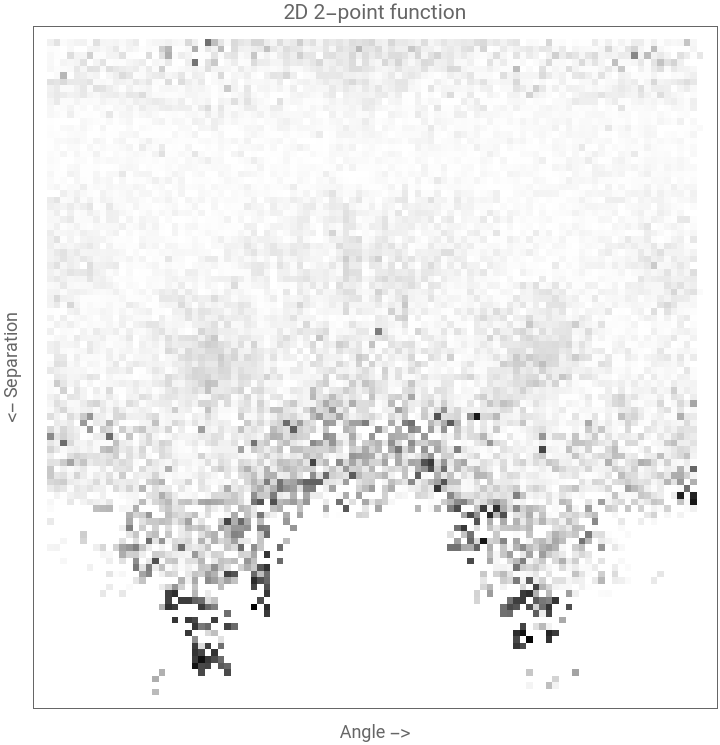
The outputs refer to the correlation function computed over 2D-hypersurfaces of the metrics analyzed. The line of sight is fixed at {0,1} for all verteces.
It’s interesting to look at the behaviour of both the 1D- and 2D- correlation cases.
First, notice that the population of pairs lowers for increasing separations as expected. The horn-shaped tails at high separation are due to the limited extension of the patches analyzed. Indeed, only pairs aligned along the two diagonals (+-45°) reach those separation values, hence the distribution is skewed in the angular direction.
The 1D statistics also shows that for high separation the number of points decreases, the variance increases and flat-spacetime is retrieved. The combination of such effects results in a boost of the correlation signal.
Below the horizon characteristic length-scale, positive correlation is retrieved due to the spatial distribution of points). Look at the Schwarzschild spatial distribution of as a visual reference.
More interestingly, both Schwarzschild and Kerr show wiggles in the correlation function just after the horizon characteristic length. This behaviour is purely due to discretization effects and must be investigated further, as it could lead to physical observational phenomena happening in the surrounding of a BH.
Schwarzschild (m=1)
Out[]=
,
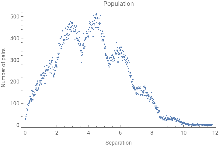
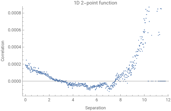
Out[]=
,
Schwarzschild (m=10)
Out[]=
,
Out[]=
,
Kerr (J=1/3)
Out[]=
,
Out[]=
,
Kerr (J=2/3)
Dimension Perturbations
Dimension Perturbations
In the graph modelling of discrete spacetime, perturbation of the graph may be introduced as single-edge removal or addition between random pair of points. This effectively can be interpreted as a local variability of the speed of light. This perturbation also changes the dimension estimation since it alters the overall number of edges.
It is then interesting to look at how these dimension perturbations evolve across known space - time structures, starting to build the framework towards actual observational predictions .
Note however that the perturbed graph does not represent a discretization of the original metric, hence it is necessary to retrieve an updated version of the metric tensor and compute the spatial hypersurfaces evolution via GRAVITAS.
In order to achieve that, here we implement a first-step approach.
We compute the Ricci curvature scalar locally at the point in which the perturbation occurs (with radius equal to the added/removed edge). The computation of the Ricci scalar curvature involves comparing the volumes of finite geodesic balls in a graph with those of finite geodesic balls of equal radius in a flat manifold. This approach serves as the discrete counterpart to the standard Ricci scalar curvature in Riemannian geometry.
Then, NSolve is used to retrieve perturbation parameters attached to the metric component to mach the Ricci scalar at that point. Naturally, the solution is not unique and many iterations of random perturbation may be tested in order to successfully get a matching between discretized perturbed metric and perturbed graph.
The code below implements this iterative procedure.
Dimension Perturbation Evolution
Dimension Perturbation Evolution
Let us investigate how a set of dimension perturbations evolve in a Schwarzschild metric.
The full version of the code is available in the attached notebook.
The visualizations are generated by post-processing the output .wxf files as in the previous cases.
All cases consider 10 steps between {0,10} coordinate time.
The following snippet visualizes the polar graphs associated to each step for a perturbed Schwarzschild graph (from a reconstructed metric).
Test Case: Pure Schwarzschild
Test Case: Pure Schwarzschild
Note that for compactness just the first and last steps are shown
One can notice that indeed the behaviour is quite stable.The variability is mainly due to the low number of points considered for the analysis, which leads to fluctuations across the time steps. One should in principle perform more fine-grained runs to resolve the features.
Indeed, also the 2D-correlation function shows almost static behaviour across the time steps.
Perturbed Schwarzschild
Perturbed Schwarzschild
Here the perturbation clearly seems to affect the correlation function at small timescales. The behaviour of the wiggle is then damped at later times, retrieving a similar structure at the final step, hinting at a dissipation of the effect.
Conclusions and Future Work
Conclusions and Future Work
Some of the features of variable dimensionality have been analyzed making use of summary statistics.
Future perspectives of this work include the extension to different metrics (FLRW and Kerr are already on the works), to address the evolution over different contexts.
The large-scale cosmological context is particularly interesting after the recent NANOGrav Collaboration results hinting at the detection of a stochastic gravitational-wave background. The scattering of this new observable with dimension waves may lead to the first indirect observational predictions of the Wolfram model.
In practice, more refined analysis must be performed with many more points.
Furthermore a formal metric reconstruction approach must be developed, analyzing the full Reimann tensor and making use of the Gauss–Codazzi equations for a fully general treatment.
Keywords
Keywords
◼
WSS23
◼
Cosmology
◼
Correlation function
◼
General relativity
◼
Black holes
◼
Wolfram model
◼
Observations
◼
Dimension perturbations
Acknowledgment
Acknowledgment
I want to deeply thank my mentors Jonathan Gorard and Nikola Bukowiecka for the chance of working on such an interesting project. I would also like to thank them for all the support, interesting conversations and late-night coding sessions.
References
References
◼
[Gorard, J.] - Non-Vacuum Solutions, Gravitational Collapse and Discrete Singularity Theorems in Wolfram Model Systems https://arxiv.org/abs/2303.07282
◼
[Gorard, J.] - Some Relativistic and Gravitational Properties of the Wolfram Model https://arxiv.org/abs/2004.14810
◼
[Gorard, J.] - Gravitas https://github.com/JonathanGorard/Gravitas
CITE THIS NOTEBOOK
CITE THIS NOTEBOOK
Cosmological imprints on the 2-point correlation function of over-dimension fields
by Federico Semenzato
Wolfram Community, STAFF PICKS, July 12, 2023
https://community.wolfram.com/groups/-/m/t/2959794
by Federico Semenzato
Wolfram Community, STAFF PICKS, July 12, 2023
https://community.wolfram.com/groups/-/m/t/2959794