CITE THIS NOTEBOOK: Control Theory for Physicists by John Bechhoefer. Wolfram Community OCT 31 2022.
ORIGINAL BOOK: Bechhoefer J. Control Theory for Physicists. Cambridge United Kingdom: Cambridge University Press, 2021. ISBN: 9780511734809. DOI: https://doi.org/10.1017/9780511734809. Amazon: https://www.amazon.com/Control-Theory-Physicists-John-Bechhoefer/dp/1107001188.
ORIGINAL BOOK: Bechhoefer J. Control Theory for Physicists. Cambridge United Kingdom: Cambridge University Press, 2021. ISBN: 9780511734809. DOI: https://doi.org/10.1017/9780511734809. Amazon: https://www.amazon.com/Control-Theory-Physicists-John-Bechhoefer/dp/1107001188.
Introduction
Introduction
This book began as an attempt by a physicist (the author) to understand control theory, a topic that is important for both technological and conceptual reasons but which lacks a place in the traditional physics curriculum. For technology, control theory is one of a very few general conceptual frameworks of engineering. It is relevant to the functioning of almost all practical devices, and will help physicists (yourself and/or your competition!) build better experiments. For theoretical physics, control theory is at the heart of Maxwell’s demon and efforts to understand the role of information in thermodynamics. It is also relevant to almost all aspects of biology, from the homeostasis of body temperature to circadian rhythms to gene expression to the complicated decisions that cells continually make. Learning about control theory is key to understanding the role of evolution (biological and technological). Thus, whether you are interested in things or theories, this book has something for you! It is first a textbook and has been used for courses at the advanced undergraduate and beginning graduate level. The book is also well-suited for self-study, as ideas are developed carefully and the presentation is self-contained. The mathematics level starts from the “Math Methods for Physics” class that most physicists take in their second or third year of undergraduate education. For non-physicists, this means a familiarity with linear differential equations, linear algebra, and Fourier transforms. Other mathematical methods are developed in the book (or summarized in the online Appendix). Very little actual physics is assumed, but the examples are ones that are familiar and interesting to physicists. But hopefully others will like them, too!
The goal then is to take a very broad view of control theory. I try to present ideas in their simplest non-trivial form, to make clear what is going on. The presentation is informal but careful. For formal theory, there are plenty of control theory books that take an applied-mathematics approach. Here the style is more that of a physics text, with an emphasis on the basic ideas and fundamental limitations. (This is one of the only books to discuss both mathematical and physical limits to control.)
In trying to explain ideas simply, I found that Mathematica is a wonderful l tool. Using both its basic functions and many control-theory special operations, one can tackle very easily and clearly a wide variety of problems. The Mathematica code is kept quite basic — one of Mathematica’s virtues is that so much is possible without the intricate and somewhat abstract programming one often sees in fancy demonstrations. Another is its ability to do both symbolic and numeric computations.
The publisher's website makes the full table of contents, preface, index, and part of the first chapter available. The online resources include an appendix of mathematical methods, statement and solution for all the problems in the book, and Mathematica notebooks supplementing the problems and examples. Below are four related examples adapted from some of those notebooks (all having to do with oscillators or pendula, stable and unstable). They give a flavor for this aspect of the book.
Part I. Undamped oscillator with PID control, for disturbance rejection & command tracking (Prob. 3.2)
Part I. Undamped oscillator with PID control, for disturbance rejection & command tracking (Prob. 3.2)
We begin by defining the dynamics of the linear system as a transfer function in the Laplace (s) domain.
In[]:=
Clear["Global`*"];tf[ζ_]:=TransferFunctionModel+2ζs+1,s(*transferfunctionofasecond-ordersystem(oscillator)withfrequency=1andscaleddampingcoefficientζ*)d=DiracDelta[t];(*d=impulseinputdisturbance*)step=UnitStep[t];(*stepinputdisturbance*)ζvals={0.01,0.3,1,3};(*valuesofdampingtouse*)trange={t,0,10};
1
2
s
We plot the time response to an impulse perturbation at t=0. Mathematica has many control-specific commands that simplify common control tasks. Here we see the response to an impulse disturbance (a “hammer hit”), which is modeled as a Dirac delta function applied to the system input. (Physically this means that the impulse is a sudden force, which affects the velocity instantaneously and the position after some time.)
In[]:=
yOpenLoop=Table[OutputResponse[tf[ζ],d,t],{ζ,ζvals}];Plot[Evaluate[yOpenLoop],trange,PlotRange->{-1,1}]
Out[]=
We can also display easily a Bode plot (frequency response, for magnitude and phase). The x-axis of the plot is angular frequency, ω.
In[]:=
BodePlot[tf[ζvals],{0.01,100}]
Out[]=
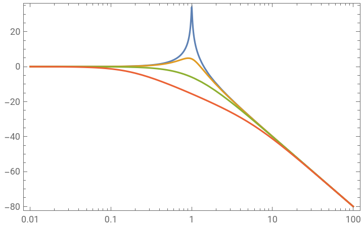
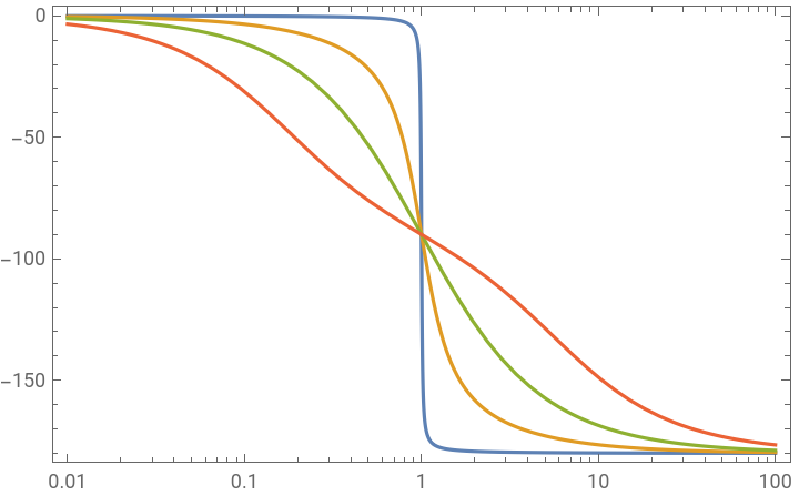
An alternate method to characterize frequency response is a Nyquist plot, which is the frequency response in the complex s-plane.
In the physics literature, the Nyquist plot is known as a “Cole-cole plot” in the context of modeling glassy dynamics (dielectric relaxation, etc.).
In the physics literature, the Nyquist plot is known as a “Cole-cole plot” in the context of modeling glassy dynamics (dielectric relaxation, etc.).
In[]:=
ζvals1=Drop[ζvals,1];(*dropzerodampingcase,awkwardtoplot*)NyquistPlot[tf[ζvals1],{0.01,100}]
Out[]=
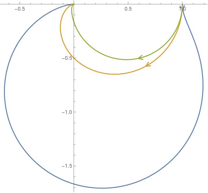
Now let us see how adding different types of control affect the undamped case (ζ=0). We begin with pure proportional control and see how it affects the response to a disturbance to the input.
That is, you “hit” the oscillator — apply an impulse force — and see what happens.
That is, you “hit” the oscillator — apply an impulse force — and see what happens.
In[]:=
G=+1;Gtf=TransferFunctionModel[G,s];K1=Kp;SG1=Together;SG1tf=TransferFunctionModel[SG1,s]
1
2
s
G
1+K1G
Out[]=

1 1+Kp+ 2 s |
In[]:=
y1=Table[OutputResponse[SG1tf,d,t],{Kp,{0,3,10,30}}];(*closed-loopforvariousKp*)Plot[Evaluate[y1],{t,0,10},PlotRange->{-1,1}]
Out[]=
In the plot above, the open-loop response is in blue. Adding proportional feedback both reduces the amplitude of oscillation and increases the frequency. Usually, this would not be a desired response.
Let us try a different strategy, derivative control, where the control signal is proportional to the derivative of the error signal.
Let us try a different strategy, derivative control, where the control signal is proportional to the derivative of the error signal.
In[]:=
K2=Kds;SG2=Together;SG2tf=TransferFunctionModel[SG2,s]
G
1+K2G
Out[]=
1 1+Kds+ 2 s |
In[]:=
y2=Table[OutputResponse[SG2tf,d,t],{Kd,{0,1,3,5}}];(*closed-loopforvariousKd*)Plot[Evaluate[y2],trange,PlotRange->{-1,1}]
Out[]=
We see that the derivative term increases the damping. That is also apparent in looking at the transfer function SG2tf between the input and output of the closed-loop dynamics. It is identical to a damped oscillator, where the damping is now provided by the derivative feedback term Kd instead of an intrinsic damping ζ.
The benefits of proportional control (faster response, reduced amplitude) and derivative control (damping) can be combined with PD control.
The benefits of proportional control (faster response, reduced amplitude) and derivative control (damping) can be combined with PD control.
In[]:=
K3=Kp+Kds;SG3=Together;SG3tf=TransferFunctionModel[SG3,s]
G
1+K3G
Out[]=
1 1+Kp+Kds+ 2 s |
In[]:=
y0=OutputResponse[SG3tf/.{Kp0,Kd0},d,trange];y3a=OutputResponse[SG3tf/.{Kp0,Kd3},d,trange];y3b=OutputResponse[SG3tf/.{Kp1,Kd3},d,trange];y3c=OutputResponse[SG3tf/.{Kp5,Kd6},d,trange];p3a=Plot[{y0,y3a,y3b,y3c},trange,PlotRange->{-1,1}]
Out[]=
PD control thus can work well against an impulse disturbance. It also helps for a step disturbance but there is always an offset.
In[]:=
y3d=OutputResponse[SG3tf/.{Kp0,Kd0},step,trange];(*openloop*)y3e=OutputResponse[SG3tf/.{Kp2,Kd3},step,trange];y3f=OutputResponse[SG3tf/.{Kp5,Kd6},step,trange];p3c=Plot[{y3d,y3e,y3f},trange,PlotRange->{0,2},GridLines->{{},{1}}]
Out[]=
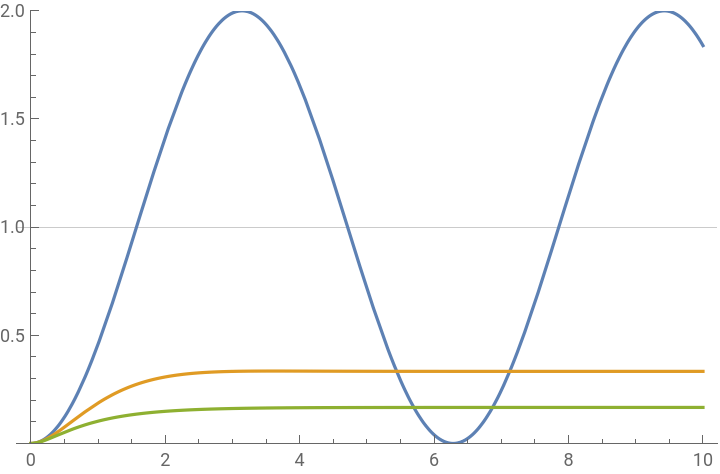
Adding an integral term to the controller (making PID control) removes the offset. Compare the open loop (blue), PD control (orange), and PID control (green) step responses.
Two final points:
(1) We have ignored noise. The derivative term, in particular, amplifies noise and this can be a reason to limit the size of Kd.
(2) We have also ignored the size of the control signal. Let’s look at it for the PID control example.
(1) We have ignored noise. The derivative term, in particular, amplifies noise and this can be a reason to limit the size of Kd.
(2) We have also ignored the size of the control signal. Let’s look at it for the PID control example.
The blue curve shows u(t) for a step response, which is quite reasonable. Notice that it asymptotes to u = –1, which is needed to counteract the imposed step amplitude of +1.
However, when the same controller is given an impulse disturbance, the required initial value of u(t) ~ –3, which is a much larger signal. The overall point is that you have to make sure that your actuator can supply the signal required by the expected commands and disturbances. If not, one solution is to design a control that takes into account the control constraint. This is done in Section 7.5. Or you can just buy a bigger actuator!
However, when the same controller is given an impulse disturbance, the required initial value of u(t) ~ –3, which is a much larger signal. The overall point is that you have to make sure that your actuator can supply the signal required by the expected commands and disturbances. If not, one solution is to design a control that takes into account the control constraint. This is done in Section 7.5. Or you can just buy a bigger actuator!
Part II. Observer-based feedback for undamped, unstable oscillator; simulate combined system (Prob. 4.9)
Part II. Observer-based feedback for undamped, unstable oscillator; simulate combined system (Prob. 4.9)
In this second example, we control an undamped system that is unstable. In contrast to the previous example, which used frequency-domain (Laplace plane) techniques, here we use state space (time-domain) techniques. For this technique, the feedback control is based on the entire internal state vector (here, θ and θd, the angular velocity). However, we only observe the position. Even so, we can estimate the velocity by constructing an observer, a computer copy of the dynamical system that uses the discrepancy between observations (y) and the expected position (x) to synchronize the observer dynamics with those of the physical system. Once the two dynamical systems are synchronized, we can read out the state estimates θh and θhd and use those in the feedback.
The blue curves are the actual state and the orange curves the estimator dynamics. Even though the initial condition for the angular-velocity estimate (right) is far off, the estimate rapidly converges to the system state.
Repeat the above more simply using the special Mathematica system command, EstimatorRegulator:
Repeat the above more simply using the special Mathematica system command, EstimatorRegulator:
As a bonus, here are a few explicit quantities (the state-space matrices, analytic solutions, and gain matrices), for reference.
Part III. LQG control of undamped, stable oscillator; simulate combined system (Prob. 8.7)
Part III. LQG control of undamped, stable oscillator; simulate combined system (Prob. 8.7)
We next consider a stochastic counterpart to the previous problem (but substituting stable for unstable dynamics).
Define the continuous system, with noisy inputs; then discretize. In this way to define the system, we can give the “classical form” of the second-order differential equation for x(t).
Define the continuous system, with noisy inputs; then discretize. In this way to define the system, we can give the “classical form” of the second-order differential equation for x(t).
The main difference between this example and the previous one is that the gains are now chosen systematically from the cost function and noise statistics. In the previous example, they were chosen heuristically. We begin with the open-loop disturbance response, using a Kalman filter to provide the state estimates. We use the prediction observer, where the estimate is based on the history up to the previous time step. This is simpler than the current estimator (discussed at length in the book), which uses observations up to the current moment. The latter gives estimates with slightly less variance (the information is more current), but the formulas are a bit more complicated and, more important, it is only relevant for slower dynamics where the computations and data processing happen much faster than the rate data are acquired.
We then combine the Kalman filter with an optimal controller, to create an “LQG” (linear quadratic Gaussian) controller for disturbance response. First, we give the explicit construction.
Graphs: Left are measurements (pink), true state (blue) and estimate (black) for the open-loop dynamics. Notice that the estimate converges much closer to the true state than the observations.
The middle plot shows the same quantities for the controlled dynamics. The right plot shows the difference between states and estimates for x, calculated for both the open and closed-loop cases (i.e, without and with feedback) . The green line at 0 shows that the two calculations give identical results, showing that the presence or absence of feedback does not affect the ability to estimate states.
The middle plot shows the same quantities for the controlled dynamics. The right plot shows the difference between states and estimates for x, calculated for both the open and closed-loop cases (i.e, without and with feedback) . The green line at 0 shows that the two calculations give identical results, showing that the presence or absence of feedback does not affect the ability to estimate states.
Finally, we compare the above explicit calculations for the closed-loop system with one using the built-in routine LQGRegulator. We also introduce sspec, an “association”, which is an alternate way to specify system properties.
The two are the same (except again for the extra input, which Mathematica uses to allow an extra “exogenous” input).
Part IV. Pendulum swing up, as a boundary-value problem (Prob. 7.18)
Part IV. Pendulum swing up, as a boundary-value problem (Prob. 7.18)
The result of the calculation is the plot below, at left. The orange curve with filling is the calculated feedforward u(t) = uff(t). It is supposed to produce the blue curve θ(t). Both curves are interpolated, so we do not see the actual grid points from the FindRoot solution.
Next, we test this approximate solution on the open-loop dynamics, integrated at a smaller time steps that are chosen adaptively by NDSolveValue. That is, we input uff(t) to the “real” (simulated) system.
Next, we test this approximate solution on the open-loop dynamics, integrated at a smaller time steps that are chosen adaptively by NDSolveValue. That is, we input uff(t) to the “real” (simulated) system.
The result is the middle plot, below. The protocol drives the pendulum to θ=π (up) at τ=5, as it was designed to do. We then continue the integration and find that eventually the pendulum falls over. The reason is that numerical error implies that we do not end up perfectly at θ=π. Because the up equilibrium is unstable, eventually that error becomes large and the pendulum falls.
We next show that adding linear feedback can stabilize against “bad” numerics. We compute the discrepancy between the actual value of the state and nominal calculated value. We can do this both during the initial protocol and afterwards. We then apply a linear feedback law (calculated from an LQR algorithm for the upright pendulum, not shown).
We next show that adding linear feedback can stabilize against “bad” numerics. We compute the discrepancy between the actual value of the state and nominal calculated value. We can do this both during the initial protocol and afterwards. We then apply a linear feedback law (calculated from an LQR algorithm for the upright pendulum, not shown).
The right-hand plot shows that with added feedback, the system can swing up and balance the pendulum. Actually the feedback can correct far larger perturbations than the small amount generated by numerical errors. This gives the feedforward + feedback algorithm nice robustness properties. Being robust against external disturbances, numerical error (and uncertainties in the exact dynamical equations) is one of the major goals of control theory.
Finally, let’s animate the pendulum swing up. To make the animation more interesting, we will first calculate a longer protocol (τ=25). Because we are minimizing control effort, the optimum solution is to swing back and forth over several cycles, adding a bit of amplitude each time. We do not include feedback, so that we can see the pendulum fall over after the protocol ends (between τ=25 and 30).
Finally, let’s animate the pendulum swing up. To make the animation more interesting, we will first calculate a longer protocol (τ=25). Because we are minimizing control effort, the optimum solution is to swing back and forth over several cycles, adding a bit of amplitude each time. We do not include feedback, so that we can see the pendulum fall over after the protocol ends (between τ=25 and 30).
Now do the animation with the new solution
In the animation, the moving red arc represents the time-dependent applied torque. Notice how the torque signal “leads” the pendulum response, because of the inertia of the latter.
Adding feedback will stabilize the pendulum at the top. You can execute “anim2” to see that.... Notice how the linear feedback couples to the numerical noise during swing up. The reason for the jerkiness in u(t) is that the feedback gains should be time dependent (even switching sign depending on whether the pendulum end is below or above the pivot), but it doesn’t. A quick fix would be to apply the feedback only after the pendulum is balanced in the up position. A better but more complicated solution would be to calculate a time-dependent linear feedback gain.
Adding feedback will stabilize the pendulum at the top. You can execute “anim2” to see that.... Notice how the linear feedback couples to the numerical noise during swing up. The reason for the jerkiness in u(t) is that the feedback gains should be time dependent (even switching sign depending on whether the pendulum end is below or above the pivot), but it doesn’t. A quick fix would be to apply the feedback only after the pendulum is balanced in the up position. A better but more complicated solution would be to calculate a time-dependent linear feedback gain.
Conclusion
Conclusion
I hope you have enjoyed these examples and that they make you more curious about what control theory has to offer! Please leave any comments in the space below.