Wolfram Cloud Document

ABSTRACT (original article): Ecosystems are commonly organized into trophic levels -- organisms that occupy the same level in a food chain (e.g., plants, herbivores, carnivores). A fundamental question in theoretical ecology is how the interplay between trophic structure, diversity, and competition shapes the properties of ecosystems. To address this problem, we analyze a generalized Consumer Resource Model with three trophic levels using the zero-temperature cavity method and numerical simulations. We find that intra-trophic diversity gives rise to “emergent competition’’ between species within a trophic level due to feedbacks mediated by other trophic levels. This emergent competition gives rise to a crossover from a regime of top-down control (populations are limited by predators) to a regime of bottom-up control (populations are limited by primary producers) and is captured by a simple order parameter related to the ratio of surviving species in different trophic levels. We show that our theoretical results agree with empirical observations, suggesting that the theoretical approach outlined here can be used to understand complex ecosystems with multiple trophic levels. CITATION (original article): Feng Z, Marsland R III, Rocks JW, Mehta P (2024), Emergent competition shapes top-down versus bottom-up control in multi-trophic ecosystems. PLOS Computational Biology 20(2): e1011675. https://doi.org/10.1371/journal.pcbi.1011675

Introduction

ODE model for ecological dynamics

In the paper, we proposed a set of coupled ODE equations for the consumer-resource dynamics of a 3-trophic-level ecosystems.

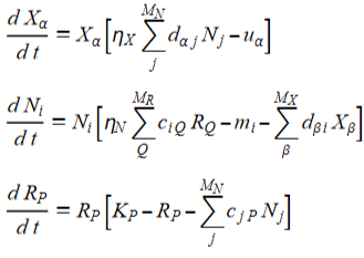
where

is a



matrix of consumer preferences for the the

primary consumers and

βi

is a



matrix of consumer preferences for the

secondary consumers, and

∈[0,1]

account for finite efficiency of biomass conversion. When

and

are close to one, energy is very efficiently transferred across trophic levels. In contrast, when these values are close to zero, energy cannot be efficiently harvested from lower trophic levels. We also define the carrying capacity

for each primary producer

, along with the death rates

for each primary consumer

and

for each secondary consumer. In this notebook, we consider the case where the consumer preferences

are drawn independently and identically with mean

and standard deviation



. We parameterize the variation in

in terms of the random variables

so that

αi



αi

>0

αi

βj

>

αβ

Similarly, we draw the consumer preferences

independently and identically with mean

and standard deviation



, parameterized in terms of the random variables



>0,



For convenience, we choose to scale the means and variances of the consumer preferences with the number of species,

. We note that this does not affect the generality of our results, but greatly simplifies the mathematical treatment in the thermodynamic limit.

Example of dynamics

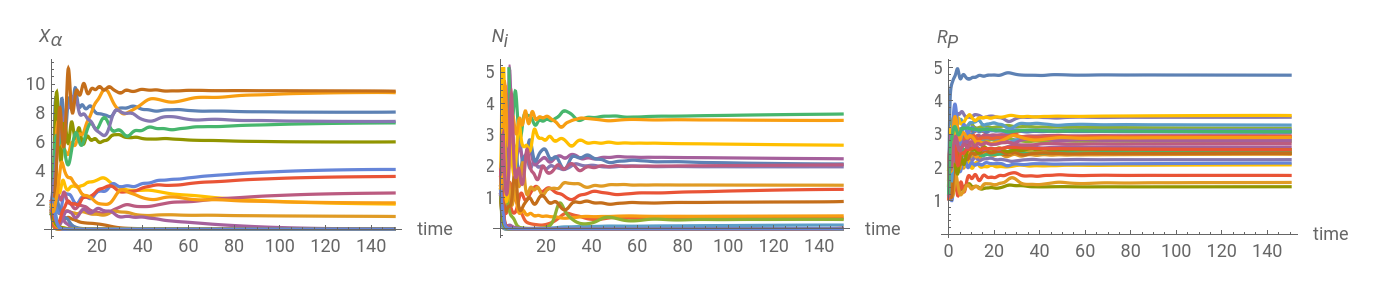
Here we choose a specific set of model parameters, define the numerical,plot one example of the dynamics. Each line represent the biomass of one species in each trophic levels.

Define function for ODE simulation

FullSimulate[topspecies_,r1_,r2_,k_,m_,u_,sigmak_,sigmam_,sigmau_,muc_,mud_,sigmac_,sigmad_,tfinal_]:=Module[{},middlespecies=Round[topspecies/r1];resources=Round[topspecies/r1/r2];iniX=RandomReal[{1,2},{topspecies}];inin=RandomReal[{1,2},{middlespecies}];iniR=RandomReal[{1,2},{resources}];Dm=RandomVariate[NormalDistribution[mud/middlespecies,sigmad/Sqrt[middlespecies]],{topspecies,middlespecies}];Cm=RandomVariate[NormalDistribution[muc/resources,sigmac/Sqrt[resources]],{middlespecies,resources}];us=RandomVariate[NormalDistribution[u,sigmau],topspecies];ms=RandomVariate[NormalDistribution[m,sigmam],middlespecies];ks=RandomVariate[NormalDistribution[k,sigmak],resources];eqns={X'[t]X[t](Dm.n[t]-us),n'[t]n[t](Cm.R[t]-ms-Transpose[Dm].X[t]),R'[t]R[t](ks-R[t]-Transpose[Cm].n[t]),X[0]==iniX,n[0]==inin,R[0]==iniR};solution=NDSolve[eqns,{X,n,R},{t,tfinal},Method"StiffnessSwitching"][[1]];AllR=Table[Evaluate[R[t]/.solution],{t,0,tfinal,0.1}];Alln=Table[Evaluate[n[t]/.solution],{t,0,tfinal,0.1}];AllX=Table[Evaluate[X[t]/.solution],{t,0,tfinal,0.1}];{AllR,Alln,AllX}];

Specify parameters for ODE simulation and make a plot of dynamics

Endtime=150;topspecies=30;sigmau=0.1;sigmam=0.1;sigmak=0.1;u=1;m=1;k=4;sigmac=0.5;muc=1;sigmad=0.5;mud=1;r1=1;r2=1;Dynamics=FullSimulate[topspecies,r1,r2,k,m,u,sigmak,sigmam,sigmau,muc,mud,sigmac,sigmad,Endtime];Rdynamics=Table[Dynamics[[1,All,alpha]],{alpha,1,Length[Dynamics[[1,1,All]]]}];Ndynamics=Table[Dynamics[[2,All,alpha]],{alpha,2,Length[Dynamics[[1,2,All]]]}];Xdynamics=Table[Dynamics[[3,All,alpha]],{alpha,3,Length[Dynamics[[1,3,All]]]}];Show[GraphicsRow[{ListLinePlot[Xdynamics,AxesLabel{"time","

"},DataRange->{0,Endtime},AspectRatio->0.5],ListLinePlot[Ndynamics,AxesLabel{"time","

"},DataRange->{0,Endtime},AspectRatio->0.5],ListLinePlot[Rdynamics,AxesLabel{"time","

"},DataRange->{0,Endtime},AspectRatio->0.5]}],ImageSize->Full]

Out[]=

Compare cavity method prediction and simulation

Self-consistency equations from cavity method

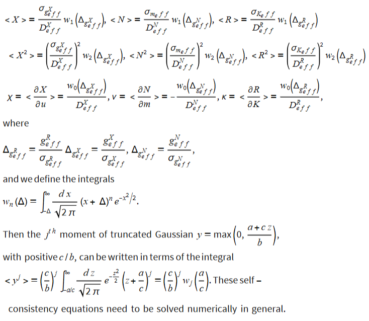
Thestatisticsofsteadystatesofthemodeldefinedintheprevioussectioncanbecalculatedusingcavitymethod.Theresultisasetofself-consistencyequationswith9equationsfor9variables,

Define functions for Gaussian integrals

Here we define the integrals for the 0, 1 and 2nd moment of truncated Gaussians as functions. We directly use the result from Integration in terms of error function speed up the code.

In[]:=

w1[d_]:=



1+Erf



2π

w0[d_]:=

1+Erf

W[d_]:=



1+Erf



2π



+(1+

)

1+Erf



Define cavity solver

We define the solver “Wholesolve” for self consistency equations from cavity method.

Plot the distribution of biomass from repeated simulations, and compare to cavity result

Plotting phase diagrams from cavity predictions

Evaluate cavity solution for a range of parameters and save the result

Here we set the range of parameters, evaluate the cavity equations in the range, and save them.

Get the effective competition and order parameters from the solutions

Making the plots

CITE THIS NOTEBOOK

Emergent competition shapes top-down versus bottom-up control in multi-trophic ecosystems
by Zhijie Feng, Robert Marsland III, Jason W. Rocks & Pankaj Mehta
Wolfram Community, STAFF PICKS, March 20, 2024
https://community.wolfram.com/groups/-/m/t/3144764