This animation uses the modular flow to produce a periodic family of Jacobi elliptic functions of type cn, visualized using domain coloring. This is also explained in my paper "Looping animations using the modular flow and elliptic functions."
ABSTRACT (original article): This paper describes an approach to generating looping animations using the modular flow and elliptic functions. The modular flow is a flow on lattices with many periodic orbits, and elliptic functions are meromorphic, doubly-periodic functions which can be visualized using domain coloring. CITATION (original article): Clayton Shonkwiler (2026), Looping Animations Using the Modular Flow and Elliptic Functions, Proceedings of Bridges 2026: Mathematics and the Arts, 533--536. http://archive.bridgesmathart.org/2026/bridges2026-533.html
The Modular Flow
The Modular Flow
See Quasi or the paper for an explanation of the modular flow. The upshot is that when is the planar lattice generated by =
and =
( is the golden ratio), and we act on the lattice points by the family of matrices
to get the family of lattices, this family turns out to be periodic with period =ln(1+ϕ):
Λ
u
1
ϕ |
1 |
u
2
1 |
-ϕ |
ϕ=
1+
5
2
t | 0 |
0 | -t |
t·Λ
t
0
In[]:=
DynamicModule[{M,pts,U={{GoldenRatio,1},{-1,GoldenRatio}}},pts=Flatten[Table[{x,y},{x,-15,15},{y,-15,15}],1];Animate[M=DiagonalMatrix[{,}].U;Graphics[{Thickness[.005],PointSize[Large],Point[M.#]&/@pts},PlotRange->10],{s,0,Log[1+GoldenRatio]},SaveDefinitions->True,AnimationRunning->False]]
s
E
-s
E
Out[]=
In particular, if has columns and and , then or, equivalently,
U
u
1
u
2
B=
2 | 1 |
1 | 1 |
diag(,)U=UB
t
0
-
t
0
diag(,)=2+
t
0
-
t
0
u
1
u
1
u
2
diag(,)=+
t
0
-
t
0
u
2
u
1
u
2
The Jacobi elliptic function
The Jacobi elliptic function
In general, elliptic functions are doubly-periodic meromorphic functions on the complex plane . The Jacobi elliptic functions are a basic family of elliptic functions of the form , where p and q are any of the letters c, s, n, or d, is the argument, and is a parameter which implicitly specifies the lattice (or, equivalently, a given lattice specifies the parameter ): for any integers and , , where is determined by p, q, , and and is the elliptic integral of the first kind. For example, for the cn function we have , so that and , and we see that the periods of cn are and .For example, is implemented in Mathematica as JacobiCN:
pq(u|m)
u
m
m
α
β
pq(u+2αK(m)+2βK(1-m)|m)=pq(u|m)
γ
(-1)
γ
α
β
K
γ=α+β
cn(u+4αK(m)|m)=cn(u|m)
cn(u+4βK(1-m)|m)=cn(u|m)
4K(m)
4K(1-m)
cn
In[]:=
ComplexPlot[JacobiCN[u,.8],{u,10}]
Out[]=
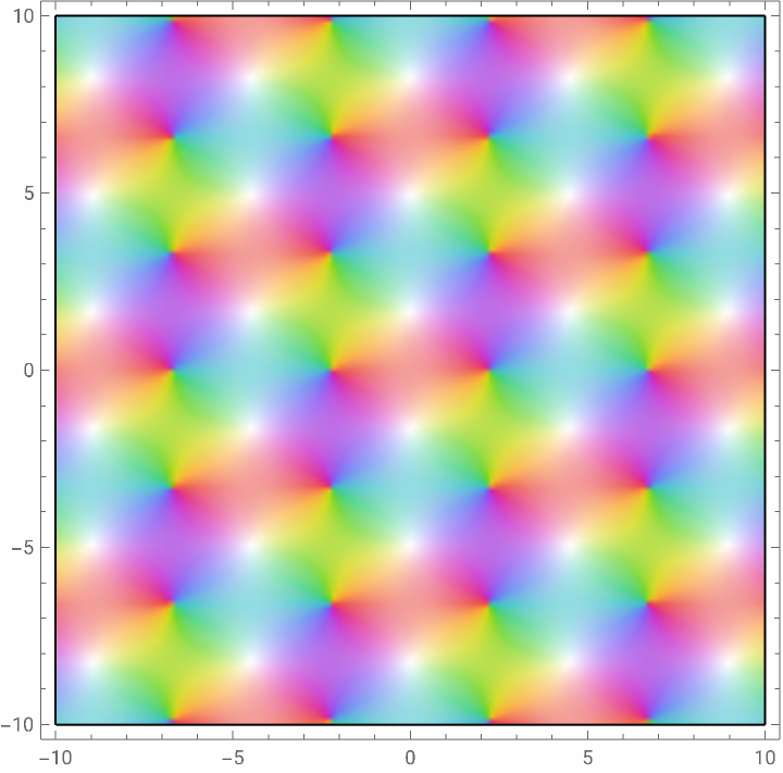
In general, will have a zero in the p corner and a pole in the q corner of the rectangle (or, more generally, parallelogram) coming from the lattice, where the corners are labeled as in this Wikipedia diagram: For this parameter , we can compute and as follows:
pq(u|m)
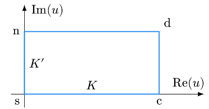
m=0.8
K(m)
K(1-m)
In[]:=
EllipticK[0.8]
Out[]=
2.25721
In[]:=
EllipticK[1-0.8]
Out[]=
1.65962
So we expect to see a (simple) zero of at and a (simple) pole at , which is indeed what we see in the plot above.
cn(·|0.8)
≈2.257
≈1.659
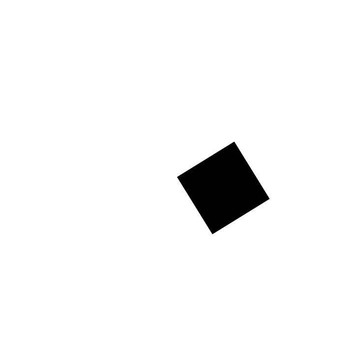
Now, the idea is that we’re going to get an animation by plotting the family of Jacobi functions, where is the family of parameters corresponding to our family of lattices. In principle, since we know the periods of cn and we know the lattice , we could try to solve for . I don’t doubt that some cleverer person than I could figure this out, but I spent a very long time trying and failing to figure this out due to the facts that: (i) has a branch cut discontinuity running from 1 to ∞ and (ii) I’m representing by and , which span an increasingly long and pointy parallelogram.
cn(·|)
m
t
m
t
t·Λ
t·Λ
m
t
K
t·Λ
t·=
u
1
t |
-t |
t·=
u
2
t |
- -t |
In[]:=
AnimateGraphicsParallelogram[{0,0},{{GoldenRatio,},{,-GoldenRatio}}],PlotRange->5,{t,0,Log[1+GoldenRatio]},SaveDefinitions->True,AnimationRunning->False
t
E
-t
E
t
E
-t
E
Out[]=
So instead I’m going to represent cn in terms of the Weierstrass -function. In general, an even elliptic function with zeros at and poles at can be represented as , where is some fixed constant (see, for example, §8.10 in Lawden’s Elliptic Functions and Applications). Since cn is even, we can use this representation. We know from the construction of cn that it should have zeros at and and poles at and , so we can just plug these into the above representation to get an alternative formula for cn.
℘
f
±,…,±
z
1
z
n
±,…,±
p
1
p
n
f(z)=a
n
∏
i=1
℘(z)-℘()
z
i
℘(z)-℘()
p
i
a
±
ω
1
4
±+
3
ω
1
4
ω
2
2
±
ω
2
4
±+
3
ω
2
4
ω
1
2
Translating to complex numbers, we saw above that after one period
In particular, our zeros and poles get sent as follows:
So we’ll need to run the modular flow for 3 periods to get a looping animation.
So here’s the code for the animation:
Which we can export to a GIF:
Or visualize using ListAnimate:
CITE THIS NOTEBOOK
CITE THIS NOTEBOOK
cn (elliptic function animation)
by Clayton Shonkwiler
Wolfram Community, STAFF PICKS, June 24, 2026
https://community.wolfram.com/groups/-/m/t/3738945
by Clayton Shonkwiler
Wolfram Community, STAFF PICKS, June 24, 2026
https://community.wolfram.com/groups/-/m/t/3738945