Liquid Liquid Equilibrium Curve and Tie Lines
for ternary system: Water + Diethyl Carbonate + Ethanol at 296.15 K
Authors: Housam Binous and Ahmed Bellagi
Liquid Liquid Equilibrium Curve and Tie Lines
for ternary system: Water + Diethyl Carbonate + Ethanol at 296.15 K
Authors: Housam Binous and Ahmed Bellagi
for ternary system: Water + Diethyl Carbonate + Ethanol at 296.15 K
Authors: Housam Binous and Ahmed Bellagi
Reference:
Housam Binous and Ahmed Bellagi, Calculation of Ternary Liquid - Liquid Equilibrium Data using Arc - Length Continuation, Engineering Reports, 3 (2), 2021.
Isabel C. Arango Montoya, Juan M. Gonzalez, and Aída L. Villa, J. Chem. Eng. Data 2012, 57, 1708−1712, Liquid−Liquid Equilibrium for the Water + Diethyl Carbonate + Ethanol System at Different Temperatures
Gas constant, temperature and binary interaction parameters for the NRTL model
param={a120.2`,a130.3,a320.2,A120.,B1213966.29,A210.,B21332.63,A130.,B132942.71,A310.,B311660.67,A230.,B236920.04,A320.,B32-774.71};
TK=296.15;
Activities using the NRTL model
GAMMA1=Exp[(t21G21x2+t31G31x3)/(x1+G21x2+G31x3)+x1/(x1+G21x2+G31x3)(-(x2t21G21+x3t31G31)/(x1+G21x2+G31x3))+x2G12/(G12x1+x2+G32x3)(t12-(x1t12G12+x3t32G32)/(G12x1+x2+G32x3))+x3G13/(G13x1+G23x2+x3)(t13-(x1t13G13+x2t23G23)/(G13x1+G23x2+x3))]/.x31-x1-x2;GAMMA1p=Exp[(t21G21xp2+t31G31xp3)/(xp1+G21xp2+G31xp3)+xp1/(xp1+G21xp2+G31xp3)(-(xp2t21G21+xp3t31G31)/(xp1+G21xp2+G31xp3))+xp2G12/(G12xp1+xp2+G32xp3)(t12-(xp1t12G12+xp3t32G32)/(G12xp1+xp2+G32xp3))+xp3G13/(G13xp1+G23xp2+xp3)(t13-(xp1t13G13+xp2t23G23)/(G13xp1+G23xp2+xp3))]/.xp31-xp1-xp2;GAMMA2=Exp[(t12G12x1+t32G32x3)/(G12x1+x2+G32x3)+x1G21/(x1+G21x2+G31x3)(t21-(x2t21G21+x3t31G31)/(x1+G21x2+G31x3))+x2/(G12x1+x2+G32x3)(-(x1t12G12+x3t32G32)/(G12x1+x2+G32x3))+x3G23/(G13x1+G23x2+x3)(t23-(x1t13G13+x2t23G23)/(G13x1+G23x2+x3))]/.x31-x1-x2;GAMMA2p=Exp[(t12G12xp1+t32G32xp3)/(G12xp1+xp2+G32xp3)+xp1G21/(xp1+G21xp2+G31xp3)(t21-(xp2t21G21+xp3t31G31)/(xp1+G21xp2+G31xp3))+xp2/(G12xp1+xp2+G32xp3)(-(xp1t12G12+xp3t32G32)/(G12xp1+xp2+G32xp3))+xp3G23/(G13xp1+G23xp2+xp3)(t23-(xp1t13G13+xp2t23G23)/(G13xp1+G23xp2+xp3))]/.xp31-xp1-xp2;GAMMA3=Exp[(t13G13x1+t23G23x2)/(G13x1+G23x2+x3)+x1G31/(x1+G21x2+G31x3)(t31-(x2t21G21+x3t31G31)/(x1+G21x2+G31x3))+x2G32/(G12x1+x2+G32x3)(t32-(x1t12G12+x3t32G32)/(G12x1+x2+G32x3))+x3/(G13x1+G23x2+x3)(-(x1t13G13+x2t23G23)/(G13x1+G23x2+x3))]/.x31-x1-x2;GAMMA3p=Exp[(t13G13xp1+t23G23xp2)/(G13xp1+G23xp2+xp3)+xp1G31/(xp1+G21xp2+G31xp3)(t31-(xp2t21G21+xp3t31G31)/(xp1+G21xp2+G31xp3))+xp2G32/(G12xp1+xp2+G32xp3)(t32-(xp1t12G12+xp3t32G32)/(G12xp1+xp2+G32xp3))+xp3/(G13xp1+G23xp2+xp3)(-(xp1t13G13+xp2t23G23)/(G13xp1+G23xp2+xp3))]/.xp31-xp1-xp2;G12=Exp[-a12t12];G21=Exp[-a12t21];G13=Exp[-a13t13];G31=Exp[-a13t31];G32=Exp[-a32t32];G23=Exp[-a32t23];t13=A13+B13/TK/8.314;t23=A23+B23/TK/8.314;t12=A12+B12/TK/8.314;t32=A32+B32/TK/8.314;t31=A31+B31/TK/8.314;t21=A21+B21/TK/8.314;
In[]:=
K={GAMMA1/GAMMA1p,GAMMA2/GAMMA2p,GAMMA3/GAMMA3p}/.param;
In[]:=
z={0.5,0.4,0.1};
In[]:=
sol=FindRoot(K[[i]]-1)z[[i]](1+(K[[i]]-1)ϕ)0,x1z[[1]](1+(K[[1]]-1)ϕ),x2z[[2]](1+(K[[2]]-1)ϕ),xp1K[[1]]z[[1]](1+(K[[1]]-1)ϕ),xp2K[[2]]z[[2]](1+(K[[2]]-1)ϕ),{ϕ,0.1},{x1,0.9},{x2,0.001},{xp1,0.004},{xp2,0.001}
3
∑
i=1
Out[]=
{ϕ0.623595,x10.903902,x20.0116968,xp10.256203,xp20.634382}
In[]:=
z={0.5,a,1-0.5-a}/.aa[s];eq1=(K[[i]]-1)z[[i]]/(1+(K[[i]]-1)ϕ)0/.x1x1[s]/.x2x2[s]/.xp1xp1[s]/.xp2xp2[s]/.ϕϕ[s];eq2=x1z[[1]]/(1+(K[[1]]-1)ϕ)/.x1x1[s]/.x2x2[s]/.xp1xp1[s]/.xp2xp2[s]/.ϕϕ[s];eq3=x2z[[2]]/(1+(K[[2]]-1)ϕ)/.x1x1[s]/.x2x2[s]/.xp1xp1[s]/.xp2xp2[s]/.ϕϕ[s];eq4=xp1K[[1]]z[[1]]/(1+(K[[1]]-1)ϕ)/.x1x1[s]/.x2x2[s]/.xp1xp1[s]/.xp2xp2[s]/.ϕϕ[s];eq5=xp2K[[2]]z[[2]]/(1+(K[[2]]-1)ϕ)/.x1x1[s]/.x2x2[s]/.xp1xp1[s]/.xp2xp2[s]/.ϕϕ[s];eq6=x1'[s]^2+x2'[s]^2+xp1'[s]^2+xp2'[s]^2+ϕ'[s]^2+a'[s]^21;derivinit={x1'[0]0,x2'[0]0,xp1'[0]0,xp2'[0]0,ϕ'[0]-0.1,a'[0]0.01};init={x1[0](x1/.sol),x2[0](x2/.sol),xp1[0](xp1/.sol),xp2[0](xp2/.sol),ϕ[0](ϕ/.sol),a[0]0.4};system=Flatten[Join[{{eq1,eq2,eq3,eq4,eq5,eq6},derivinit,init}]];
3
∑
i=1
In[]:=
SOL=NDSolve[system,{x1,x2,xp1,xp2,ϕ,a},{s,-5.5,1},AccuracyGoal->3]

Out[]=
x1InterpolatingFunction,x2InterpolatingFunction,xp1InterpolatingFunction,xp2InterpolatingFunction,ϕInterpolatingFunction,aInterpolatingFunction


In[]:=
upbound=SOL[[1]][[1]][[2]][[1]][[1]][[2]]lobound=SOL[[1]][[1]][[2]][[1]][[1]][[1]]
Out[]=
0.872675
Out[]=
-5.5
In[]:=
DATA1=Table[{x1[s],1-x1[s]-x2[s],x2[s]}/.SOL,{s,lobound,upbound,0.001}];DATA2=Table[{xp1[s],1-xp1[s]-xp2[s],xp2[s]}/.SOL,{s,lobound,upbound,0.001}];
In[]:=
p1=TernaryListPlot[{Flatten[DATA1,1],Flatten[DATA2,1]},Joined->True,PlotStyle->Thick,GridLines->Automatic,FrameLabel->{"WATER","ETHANOL","DEC"},PlotRange->All,Method->{"Backdrop"LightBlue}]
Out[]=
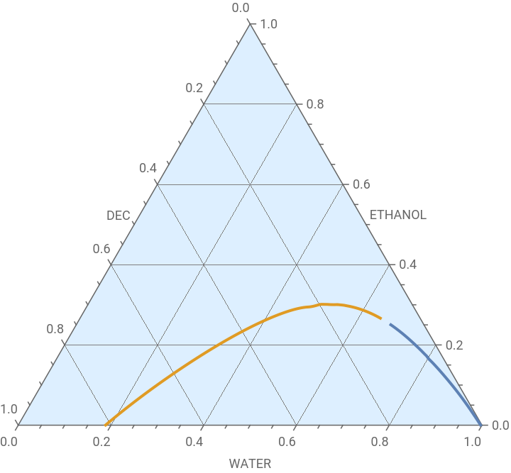
Tie Lines for Water + Diethyl Carbonate + Ethanol at 296.15 K obtained from Isabel C. Arango Montoya et al.
In[]:=
dataexp={{0.9415,0.0107,0.2439,0.733},{0.8976,0.0111,0.2697,0.6243},{0.8688,0.0117,0.309,0.5221},{0.8426,0.0161,0.3442,0.4363},{0.8223,0.0197,0.3828,0.3652},{0.7912,0.0276,0.4488,0.271},{0.9925,0.0075,0.2134,0.7866}}
Out[]=
{{0.9415,0.0107,0.2439,0.733},{0.8976,0.0111,0.2697,0.6243},{0.8688,0.0117,0.309,0.5221},{0.8426,0.0161,0.3442,0.4363},{0.8223,0.0197,0.3828,0.3652},{0.7912,0.0276,0.4488,0.271},{0.9925,0.0075,0.2134,0.7866}}
In[]:=
Pt={{2,1},{0,Sqrt[3.]}}/2;
In[]:=
data1=Table[Pt.{dataexp[[i]][[1]],1-dataexp[[i]][[2]]-dataexp[[i]][[1]]},{i,1,Length[dataexp]}]
Out[]=
{{0.9654,0.041396},{0.94325,0.0790681},{0.92855,0.10349},{0.91325,0.122369},{0.9013,0.136832},{0.8818,0.156924},{0.9925,0.}}
In[]:=
data2=Table[Pt.{dataexp[[i]][[3]],1-dataexp[[i]][[4]]-dataexp[[i]][[3]]},{i,1,Length[dataexp]}]
Out[]=
{{0.25545,0.0200052},{0.3227,0.0917987},{0.39345,0.146272},{0.45395,0.190093},{0.5088,0.218238},{0.5889,0.24266},{0.2134,2.4037×}}
-17
10
In[]:=
pexp=ListPlot[{data1,data2},PlotMarkers{Style["▲",Blue,14],Style["▲",Magenta,14]}];
In[]:=
Show[p1,pexp]
Out[]=
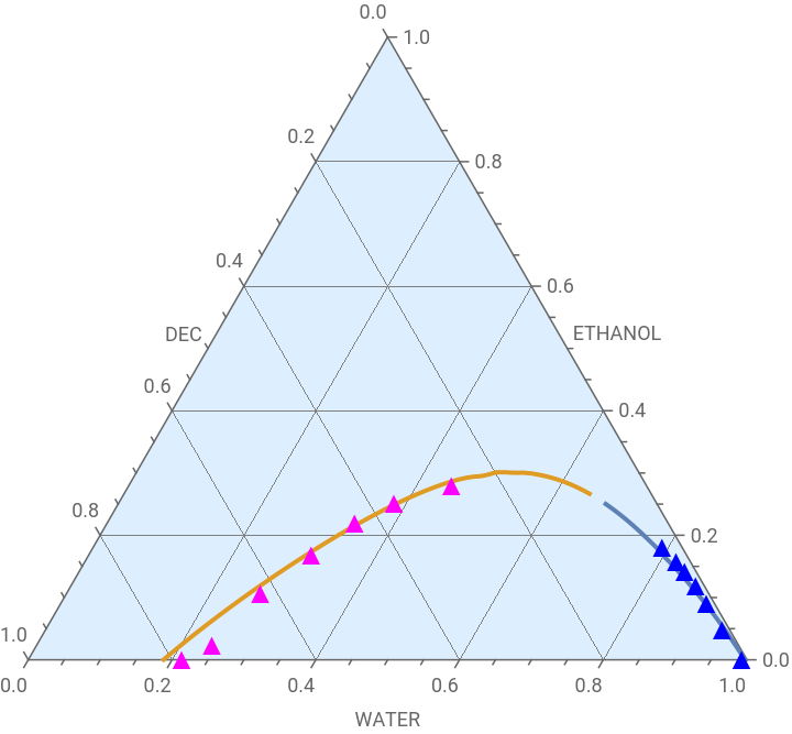
Tie Lines for Water + Diethyl Carbonate + Ethanol at 296.15 K obtained using LINGO.