Let us consider a ternary mixture of chloroform, acetone, and methanol at . The vapor-liquid equilibrium (VLE) behavior is described by the modified Raoult's law with activity coefficients predicted by the Wilson model [1]. We construct the branches of solutions for all binary and ternary azeotropes on a composition equilateral triangular diagram analogous to Fig. 7 given below and reproduced from Ref. 1.This mixture presents seven azeotropes, whose locations and boiling points are given below:
101.325kPa
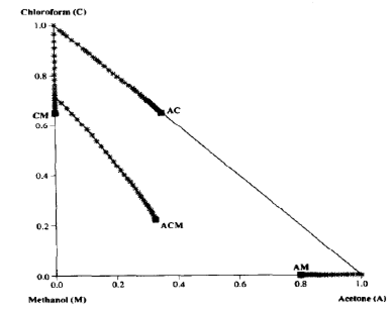
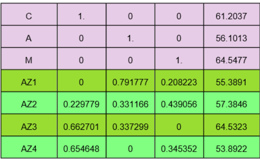
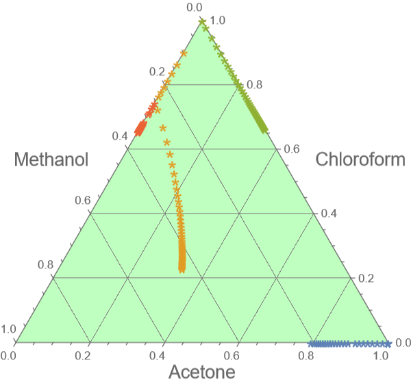
This problem was treated by Fidkowski, Malone and Doherty (Ref. 1) and their results are reproduced below:All four branches stem from the pure component corners as evidenced by our calculation:

Chloroform = component 1
Acetone = component 2
Methanol = component 3
Acetone = component 2
Methanol = component 3
Total pressure (1 atm) in torr
In[]:=
P=760;
Wilson model
In[]:=
l12=-506.85180;l21=116.11710;l13=-361.79440;l31=1694.02400;l23=-124.93280;l32=551.45450;lambdas=Transpose@{{0,l12,l13},{l21,0,l23},{l31,l32,0}};(*incal/mol*)volumes={80.7,74.0,40.7};(*inmL/mol*)wilson[x_,T_]:=Module[{Lambdas,gammas,i,j},For[i=1,i≤3,i++,For[j=1,j≤3,j++,Lambdas[i,j]=volumes[[j]]/volumes[[i]]*Exp[-lambdas[[j,i]]/(1.9872041*T)]]];For[i=1,i≤3,i++,gammas[i]=1-Log[Sum[Lambdas[i,k]x[[k]],{k,1,3}]];For[j=1,j≤3,j++,gammas[i]=gammas[i]-Lambdas[j,i]x[[j]]/Sum[Lambdas[j,k]x[[k]],{k,1,3}]]];Table[Exp[gammas[i]],{i,1,3}]]
Vapor pressure obtained using Antoine equation
In[]:=
A2=7.11714;B2=1210.595;C2=229.664;A1=6.95465;B1=1170.966;C1=226.232;A3=8.08097;B3=1582.271;C3=239.726;myPsats={10^(A1-B1/(C1+(T-273.15))),10^(A2-B2/(C2+(T-273.15))),10^(A3-B3/(C3+(T-273.15)))};
System of algebraic equations, which solutions yield the azeotropes compositions and boiling point when λ=1
mysyshom[x_,T_,l_]:=Module[{gammas,psat},gammas=wilson[x,T];psat=myPsats;{x[[1]]-((1-l)+lgammas[[1]])psat[[1]]x[[1]]/P0,x[[2]]-((1-l)+lgammas[[2]])psat[[2]]x[[2]]/P0,x[[3]]-((1-l)+lgammas[[3]])psat[[3]]x[[3]]/P0,x[[1]]+x[[2]]+x[[3]]-10}]
Compute the Jacobian matrix
In[]:=
x={x1,x2,x3};l=.;(*lisλ*)gammas=wilson[x,T];psat=myPsats;jac=Outer[D,{x[[1]]-((1-l)+lgammas[[1]])psat[[1]]x[[1]]/P,x[[2]]-((1-l)+lgammas[[2]])psat[[2]]x[[2]]/P,x[[3]]-((1-l)+lgammas[[3]])psat[[3]]x[[3]]/P,x[[1]]+x[[2]]+x[[3]]-1},{x1,x2,x3,T}];
Starting with the pure component mixture and track bifurcations
1st branch
1st branch
In[]:=
j=0;guessI={10^-12,1.0,10^-12,350};While[j≤501,k=1;guess=If[j0,guessI,guess];s=Quiet@FindRoot[mysyshom[{x1,x2,x3},T,(j)0.002],{x1,guess[[1]]},{x2,guess[[2]]},{x3,guess[[3]]},{T,guess[[4]]},MaxIterations10000];sol[j,1,1]=x1/.s;sol[j,2,1]=x2/.s;sol[j,3,1]=x3/.s;sol[j,4,1]=T/.s;jacs[j]=jac/.x1sol[j,1,1]/.x2sol[j,2,1]/.x3sol[j,3,1]/.Tsol[j,4,1]/.l(j)0.002;If[j>2&&Sign[Det[jacs[j]]Det[jacs[j-1]]]<0,Print[j];eval=Eigenvalues[jacs[j]];pos=First@Position[Abs@eval,Min[Abs@eval]];evect=Flatten[Re[Eigenvectors[jacs[j]][[pos]]]];diff={0,0,0};inc=Exp@0.01;guess={x1,x2,x3,T}/.x1sol[j,1,1]/.x2sol[j,2,1]/.x3sol[j,3,1]/.Tsol[j,4,1];Print[Sign[Det[jacs[j]]Det[jacs[j-1]]]," ",pos," ",guess];k=1;While[Abs[diff[[1]]]<10^-3&&Abs[diff[[2]]]<10^-3&&Abs[diff[[3]]]<10^-3,{guess=Re@(guess+(incevect));s=Quiet@FindRoot[mysyshom[{x1,x2,x3},T,(j+1)0.002],{x1,guess[[1]]},{x2,guess[[2]]},{x3,guess[[3]]},{T,guess[[4]]},MaxIterations10000];nbw[1]=x1/.s;nbw[2]=x2/.s;nbw[3]=x3/.s;nbw[4]=T/.s;inc=-1.5inc;diff=Table[sol[j,i,1]-nbw[i],{i,1,3}],k++}];Table[sol[j,i,1]=nbw[i],{i,1,4}];];If[j≥2&&k≥2,Table[guess[[i]]=nbw[i],{i,1,4}],Table[guess[[i]]=sol[j,i,1],{i,1,4}]];j++]
260
-1 {4} {1.17502×,1.,3.88797×,329.251}
-25
10
-27
10
261
-1 {4} {-8.62817×,0.998016,0.00198375,329.251}
-32
10
In[]:=
dataaz1=Table[{sol[j,2,1],sol[j,1,1],sol[j,3,1]},{j,0,500,10}];
2nd branch
2nd branch
In[]:=
Clear[j,guessI,s,sol,jacs,eval,evect,pos,diff,inc,nbw,k]
In[]:=
j=0;guessI={1.0,10^-12,10^-12,350};While[j≤501,k=1;guess=If[j0,guessI,guess];s=Quiet@FindRoot[mysyshom[{x1,x2,x3},T,(j)0.002],{x1,guess[[1]]},{x2,guess[[2]]},{x3,guess[[3]]},{T,guess[[4]]},MaxIterations10000];sol[j,1,1]=x1/.s;sol[j,2,1]=x2/.s;sol[j,3,1]=x3/.s;sol[j,4,1]=T/.s;jacs[j]=jac/.x1sol[j,1,1]/.x2sol[j,2,1]/.x3sol[j,3,1]/.Tsol[j,4,1]/.l(j)0.002;If[j>=2&&Sign[Det[jacs[j]]Det[jacs[j-1]]]<0,Print[j];eval=Eigenvalues[jacs[j]];pos=First@Position[Abs@eval,Min[Abs@eval]];evect=Flatten[Re[Eigenvectors[jacs[j]][[pos]]]];diff={0,0,0};inc=0.01;guess={x1,x2,x3,T}/.x1sol[j,1,1]/.x2sol[j,2,1]/.x3sol[j,3,1]/.Tsol[j,4,1];Print[Sign[Det[jacs[j]]Det[jacs[j-1]]]," ",pos," ",guess];k=1;While[Abs[diff[[1]]]<10^-3&&Abs[diff[[2]]]<10^-3&&Abs[diff[[3]]]<10^-3,{guess=Re@(guess+(incevect));s=Quiet@FindRoot[mysyshom[{x1,x2,x3},T,(j+1)0.002],{x1,guess[[1]]},{x2,guess[[2]]},{x3,guess[[3]]},{T,guess[[4]]},MaxIterations10000];nbw[1]=x1/.s;nbw[2]=x2/.s;nbw[3]=x3/.s;nbw[4]=T/.s;inc=-1.5inc;diff=Table[sol[j,i,1]-nbw[i],{i,1,3}],k++}];Table[sol[j,i,1]=nbw[i],{i,1,4}];];If[j≥2&&k≥2,Table[guess[[i]]=nbw[i],{i,1,4}],Table[guess[[i]]=sol[j,i,1],{i,1,4}]];j++]
12
-1 {4} {1.,8.27748×,-4.71551×,334.354}
-197
10
-187
10
3rd branch
3rd branch
4th branch
4th branch
All four branches of solution azeotropes on a composition equilateral diagram
References
References
◼
[1] Z.T. Fidkowski, M.F. Malone, M.F. Doherty, Computing azeotropes in multicomponent mixtures, Computers & Chemical Engineering, Volume 17, Issue 12, 1993, Pages 1141-1155, https://doi.org/10.1016/0098-1354(93)80095-5
CITE THIS NOTEBOOK
CITE THIS NOTEBOOK
Branches of solutions for azeotropes on a composition triangle: chloroform - acetone - methanol system
by Housam Binous and Ahmed Bellagi
Wolfram Community, STAFF PICKS, June 23, 2025
https://community.wolfram.com/groups/-/m/t/3483909
by Housam Binous and Ahmed Bellagi
Wolfram Community, STAFF PICKS, June 23, 2025
https://community.wolfram.com/groups/-/m/t/3483909