Understanding the Probability of Ruin with Win Rate Variations
Abstract
This computational essay looks at the classic Gambler’s Ruin problem. It studies the chance of going bankrupt and the expected length of the game for a gambler with a starting amount and a target amount. We use formulas and simulations together to check the results, and graphs show how the chance of ruin changes with the win probability. By exploring different starting and target amounts with interactive plots, we can see how the game settings affect the outcomes. This shows how theory, simulation, and visualization work together to help us understand random processes.
This computational essay looks at the classic Gambler’s Ruin problem. It studies the chance of going bankrupt and the expected length of the game for a gambler with a starting amount and a target amount. We use formulas and simulations together to check the results, and graphs show how the chance of ruin changes with the win probability. By exploring different starting and target amounts with interactive plots, we can see how the game settings affect the outcomes. This shows how theory, simulation, and visualization work together to help us understand random processes.
1. Background
The Gambler’s Ruin problem shows the risk of going bankrupt in a random process. It models a gambler who plays a game many times with a fixed chance of winning each round, starting with some money and trying to reach a target amount. In each round, the gambler either wins or loses a fixed amount, and the game continues until the gambler reaches the target or loses all their money. This problem helps us understand how the chance of winning, the starting money, and the target money together affect the risk of going bankrupt, even when the game is fair and winning and losing are equally likely.
2. Basic Idea
2.1 Core Concept
2.1 Core Concept
The main goal is to find out how likely it is that the gambler will lose all their money before reaching the target. This means looking at how the starting money, the target money, and the chance of winning each round work together to affect the risk of going bankrupt. By understanding this, we can see how vulnerable the gambler is and how small changes in the game can change the chances of reaching the goal or losing everything.
2.2 Analytical Approach
2.2 Analytical Approach
The analytical approach uses math formulas to find the exact chances of going bankrupt. In a fair game, where winning and losing are equally likely, the probability of ruin is a simple straight-line relationship between the starting money and the target money. In biased games, where the chance of winning is not 50%, a more general formula is used to consider the difference between winning and losing. These formulas let us calculate the risk of ruin exactly and show how the starting money, target money, and win probability affect the gambler’s chance of reaching the goal or going bankrupt.
3. Methodology
3.1 Simulation Implementation
3.1 Simulation Implementation
To empirically estimate the gambler’s ruin probability, we simulate the game multiple times. Each simulation starts with a given initial capital A0, continues until the gambler either goes bankrupt (0) or reaches the target B, and records the outcome. By repeating this process across many trials, we can approximate the probability of ruin and success.
The formula for the ruin probability comes from looking at the game step by step. Let R(A) be the chance that the gambler goes bankrupt when starting with capital A. In each round, the gambler either wins (gains 1 unit with probability p) or loses (loses 1 unit with probability q = 1 - p).
The formula for the ruin probability comes from looking at the game step by step. Let R(A) be the chance that the gambler goes bankrupt when starting with capital A. In each round, the gambler either wins (gains 1 unit with probability p) or loses (loses 1 unit with probability q = 1 - p).
The probability R(A) satisfies a simple recurrence:
R(A) = p * R(A + 1) + q * R(A - 1)
with boundary conditions:
R(0) = 1 (if the gambler has no money, ruin is certain)
R(B) = 0 (if the gambler reaches the target B, ruin will not happen)
By solving this recurrence with these boundaries, we can derive the closed-form formula used in the code:
R(A) = ((q/p)^A - (q/p)^B) / (1 - (q/p)^B) for p ≠ 0.5
R(A) = 1 - A/B for p = 0.5
This closed-form expression directly gives the probability of eventual bankruptcy for any initial capital, target capital, and win probability, without needing to simulate the game.
In[]:=
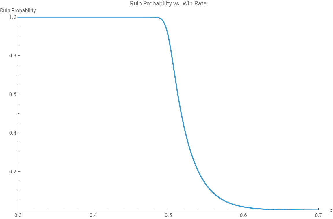
RuinProbability[A_, B_, p_] := Module[{q}, q = 1 - p; If[p == q, 1 - A/B, (* fair game: p = 0.5 *) ((q/p)^A - (q/p)^B)/(1 - (q/p)^B) (* unfair game: p ≠ 0.5 *) ]];ExpectedDuration[A_, B_, p_] := Module[{q}, q = 1 - p; If[p == q, A*(B - A), (* fair game: p = 0.5 *) (A/(q - p)) - (B/(q - p)) * ((1 - (q/p)^A)/(1 - (q/p)^B)) (* unfair game: p ≠ 0.5 *) ]];SimulateGambler[A0_, B_, p_, trials_ : 10000] := Module[{simulateOne, results}, simulateOne := Module[{A = A0}, While[A > 0 && A < B, A += If[RandomReal[] < p, 1, -1];]; A]; results = Table[simulateOne, {trials}]; <|"RuinProbability" -> Count[results, 0]/trials, "SuccessProbability" -> Count[results, B]/trials|>]SimulateGambler[10, 100, 0.5, 5000]Plot[RuinProbability[10, 100, p], {p, 0.3, 0.7}, PlotLabel -> "Ruin Probability vs. Win Rate", AxesLabel -> {"p", "Ruin Probability"}, PlotRange -> {0, 1}]
Out[]=
RuinProbability,SuccessProbability
559
625
66
625
Out[]=
3.2 Interactive Exploration
3.2 Interactive Exploration
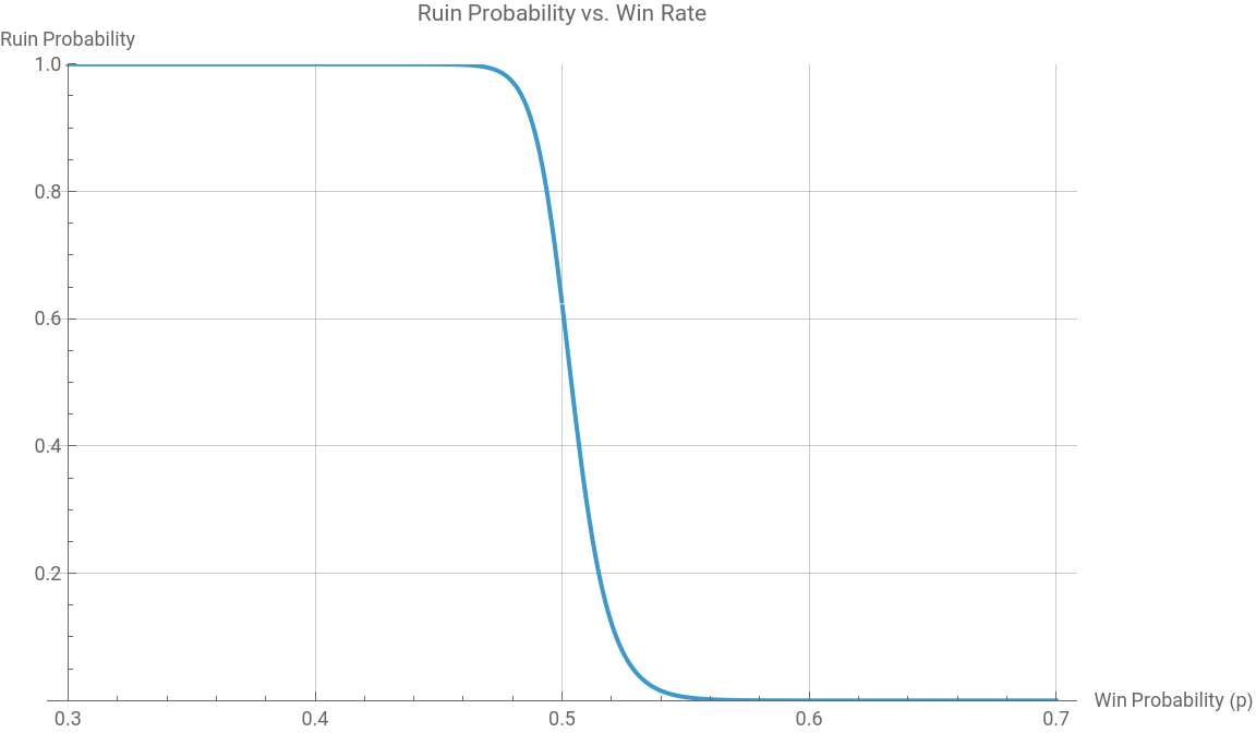
To better understand the gambler’s ruin problem, we use an interactive plot with the win probability (p) on the x-axis. The Manipulate function lets users change the starting money (A) and the target money (B) using sliders. The plot shows how the chance of going bankrupt changes with different win probabilities, making it easy to see how the starting and target money affect the gambler’s risk.
In[]:=
Manipulate PlotRuinProbability[A, B, pWin], {pWin, 0.3, 0.7}, , {A, 1, 50, 1}, (* Initial capital slider *) {B, 10, 100, 1}, (* Target capital slider *) SaveDefinitions->True
Out[]=


4. Conclusion
The Gambler’s Ruin problem shows how the risk of going bankrupt depends on the starting money, the target amount, and the chances of winning. Using both the formula and simulations, we can see how likely it is for a gambler to lose everything. Even when the chances of winning and losing are equal, the probability of ruin can still be high. Even small changes in the win probability can make a big difference in the chance of ruin. This problem is a simple example of how probability and random events affect the results in repeated games.